OR notes
Trying to understand and predict reality is one of humanity’s dreams. Nevertheless, reality is sometimes complex (see note 1), and it is therefore difficult to understand all of it with a single model. Hence, we must divide reality into different pieces that can be interpreted and obtain a partial explanation of the target. As a result, different scientific disciplines have been created to try to explain different phenomena using various models and, if possible, predict the behavior of the target subsystem.
Operations Research (see note 2) (OR) uses a set of methodologies to construct models to represent the reality to try to understand and anticipate some of the system problems. Models are tools for conceptualizing reality. Therefore, they simplify system compression and analysis. Computers were the main tool that allowed OR to develop. Many of the methods require large amounts of calculations, which in most cases are repetitive. With the help of computers, the quantity and quality of the problems solved by OR grew, which expanded the use of the discipline.
In applying these new methodologies, the relationships between different system elements are reproduced and a set of simplification hypotheses can be used (see note 3).
Notes:
- Some authors remarks that sometimes, complex behaviors are based in very simple rules: "(...) whenever a phenomenon is encountered that seems complex it is taken almost for granted that the phenomenon must be the result of some underlying mechanism that is itself complex. But my discovery that simple programs can produce great complexity makes it clear that this is not in fact correct." (Wolfram 2002). In the other hand, other authors reviewing that book (Kurzweil 2002) remark that reality is more complex that Wolfram suggest “The order of complexity of a human is greater than the interesting but ultimately repetitive (albeit random) patterns of a Class 4 automaton”. Anyway, we do not want to enter in the discussion about if the reality, or the perception of this reality, is complex or not, only to note that for us sometimes this reality is very complex.
- Operations research is traditionally considered to have emerged in the military during World War II. The initial goal of this research was to optimize military resources during the conflict. The discipline development can be said to have begun as early as the beginning of the industrial revolution. Due to the growing complexity of the organizations that replaced traditional craftspeople, new problems appeared, such as production planning problems. These problems allowed this new discipline to develop.
- Simplification hypotheses are not true in the system but are used in the construction of the model to simplify the modeling process (and sometimes just to make this process possible, due to the inherent complexity of the system).
References
Kurzweil, Ray. 2002, Reflections on Stepehn Wolfram’s ‘A New Kind of Science’ , http://www.kurzweilai.net/articles/art0464.html?printable=1 (accessed 4 January 2007)
Wolfram, Stephen 2002, A new Kind of Science, Wolfram Media, Inc.
Stochastic models
What means "Stochastic"?, basically being or having a random variable.
A stochastic model, as a model is a tool for estimating probability distributions of potential outcomes allowing random variations in one or more inputs over time. To obtain the behaviour if this random variation usually historical data for a selected period is used.
Examples of sthocastic models can be the simulation models, the queueing models and the markov chains.
Queueing models
A queueing model, in the scope of the queueing theory, is used to approximate a real queueing system in order to allow its mathematical analisys. Queueing models allow a number of useful steady state performance measures to be determined, including:
- The average number (of entities to be serverd) in the queue, or the system.
- The average time spent (by the entities) in the queue, or the system.
- The statistical distribution of the arrivals and the service times.
- The probability the queue is full, or empty.
- The probability of finding the system in a particular state.
These performance measures are important as issues or problems caused by queueing situations are often related to customer dissatisfaction with service or may be the root cause of economic losses in a business. Analysis of the relevant queueing models allows the cause of queueing issues to be identified and the impact of proposed changes to be assessed.
Markov models
In mathematics, a Markov chain, (see note 1), is a stochastic process with the Markov property (see note 2).
Future states will be reached through a probabilistic process instead of a deterministic one. At each step the system may change its state from the current state to another state, or remain in the same state, according to a certain probability distribution.
The changes of state are called transitions, and the probabilities associated with various state-changes are called transition probabilities.
Notes:
- Andrey (Andrei) Andreyevich Markov (June 14, 1856 N.S. – July 20, 1922) was a Russian mathematician. He is best known for his work on theory of stochastic processes. His research later became known as Markov chains.
- Having the Markov property means that, given the present state, future states are independent of the past states. In other words, the description of the present state fully captures all the information that could influence the future evolution of the process.
Simulation
Shannon offered a good definition of simulation: "We will define simulation as the process of designing a model of a real system and conducting experiments with this model for the purpose of understanding the behavior of the system and/or evaluating various strategies for the operation of the system.” (Shannon 1998).
These relationships and hypotheses (see note 1) describe the behavior of the system and an experimental environment that represents the target of the study is created. The various relationships and rules, which are usually mathematical (see note 2) or logical, make up the model, the tool that acquires data and provides answers about the system.
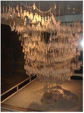
Figure 1: Model of the Sagrada Família.
Gordon (1978) establishes a classification of the models shown in the next figure.

Figure 2: Types of models (Gordon 1978)
Because of the structure of the model rules, the way they are implemented and the elements involved, different criteria can be defined to classify simulation models.
In person-to-person simulations, the model is based on individuals that play different roles. Social simulations are one example. The purpose of this kind of study is usually to analyze the reactions of individuals or groups. Job interview training is a more specific example.
Another kind of simulation involves the physical reproduction of a system. Under controlled conditions, a scale model of the system is constructed (Figure 1 shows a physical reproduction of the crypt of the Sagrada Familia temple in Barcelona).
Another kind of simulation is based on person-to-computer models.In these models, a person answers questions posed by a computer.Examples include training through financial strategy games, flight simulators, etc.
Finally, computer simulation models usually do not require user intervention. A computer program (set of decision rules) transforms input and obtains output. The category of computer simulation models can be divided into subcategories based on the set of techniques applied in the construction of the model:
- Monte Carlo simulations: The Monte Carlo method provides approximate solutions to a variety of mathematical problems by performing statistical sampling experiments on a computer. Remarkably, the method applies to problems with absolutely no probabilistic content as well as to those with inherent probabilistic structure (Fishman 1996).
- Continuous simulations: These models are characterized by the representation of the evolution of the variables of interest in a continuous way. In general this method uses ordinary differential equations if a evolution of a characteristic over the time is considered, or partial derivate equations is the evolution over space are considered too (Guasch, Piera et al. 2002).
- Discrete events: In these models, time proceeds in discrete time steps. States variables change its value in no periodic time moments. This moments are related with the event occurrence (Guash, Piera et al. 2002).
- MAS: Multi-agent systems involve a set of intelligent agents. Based on the interaction of these agents, a complex behavior emerges. Agents are fundamentally different from software packages and other commercial programs. They must have special characteristics or attributes (adaptability, mobility, transparency and accountability, ruggedness, slf-starters, user centered) (Murch and Johnson 1999).
Other classifications are presented in the next table depending on different criteria (Guash et al. 2002)
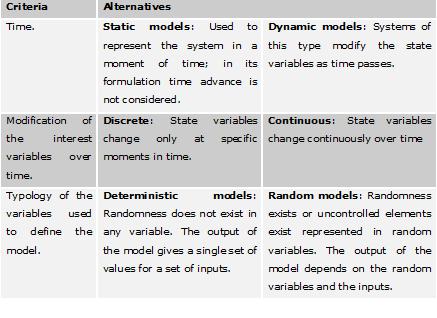
Table 1: Models classification.
Others classifications exists, for instance a classification of the modeling languages in five categories CT, CT+, DE, DE+, and CT/DE where CT means continuous time, DE discrete-event and DT discrete-time, (Beek and Rooda 1998) can be reviewed.
Methodologies based on discrete events (activity scanning, process interaction and, more specifically, event scheduling) allows us to obtain a very accurate level of detail in order to study industrial problems.
However, interest has increasingly focused on the study and analysis of systems with rich behavior that result from the interaction of complex entities and the observation of how these interactions modify the main
modeling process.
Notes:
Simplification hypotheses are not true in the system but are used in the construction of the model to simplify the modeling process (and sometimes just to make this process possible, due to the inherent complexity of the system).
Modeling using differential equations was traditionally one of the most common methodologies for studying different systems. The need for more detail made mathematical models more complex, which made construction difficult in two ways. The first was a modeling problem: there were more differential equations and more relationships between the equations. The second problem related to computing solutions: as the number of differential equations increased, the solution became more difficult and was sometimes impossible.
References
Beek, D.A. van; Rooda, J.E. 1998, Languages and applications in hybrid modelling: positioning of chi, Proc. 9th Symposium on Information Control in Manufacturing, Vol. II, Nancy, 1998, pp. 77-82.
Fishman, George S., 1996, Monte Carlo: Concepts, Algorithms and Applications, Springer, 698 pages, ISBN 038794527X
Gordon, Geoffrey, 1978, System simulation, Ed. Prentice Hall Inc, Englewood Cliffs, New Jersey 07632
Guasch, Antoni; Piera, Miquel Àngel; Casanovas, Josep; Figueres, Jaime. 2002. Modelado y simulación. Aplicación a procesos logísticos de fabricación y servicios. Edicions UPC.
Murch, Richard.; Johnson, Tony. 1999, Intelligent software agents, Prentice Hall PTR, ISBN 0-13-011021-3
Shannon, Robert E. 1998. Introduction to the art and science of simulation, Proceedings of the 1998 Winter Simulation Conference.
Discrete paradigms
SIMULATION DISCRETE PARADIGMS
Pau Fonseca i Casas; pau@fib.upc.edu
Discrete simulation paradigms
Event Scheduling
Programació
d’esdeveniments (PE) Programación de eventos.
Process interaction
Interacció
de processos (IP) Interacción de procesos.
Activity scanning
Exploració
d’activitats (EA) Exploración de actividades.
ES: example
Time between arrivals a1 35 a2 a3 a4 12 29 47 Service time b1 b2 b3 b4 40 30 30 20
a5
12
b5
30
ES: chronogram
End of service (Exits)
A1 A2 A3
Server Server occupation
S2
S1
S3
Queue New clients
A2 A3 A4 A5
0
A1
35
12
29
47
12
Time
ES: Event list
event
event
event
event
event struct { Execution time: real Priority: enter Kind: enter } End struct
ES: event
Kind of event
Depends on the model definition. Exit event, enter event for a MM1 queue. Shows the time when the event enters in the simulation system. Shows when the simulation engine must run the event.
Creation time
Running time
Priority
ES: event
The time when the simulation engine runs the event. Priority must be taken in consideration only if two ore more) events have the same run time. The Kind of event allows to define the procedure that the simulation engine must run when the event is exe
ES
Simulation clock initialization.
Model initialization.
End of simulation?
Take the first event of the event list.
Run the event
Update the clock depending on the run time of the event.
Events list Statistical data preparation. Write the results.
ES: Arrive event procedure
Generation of the next arrival
Is the machine free?
Queue ++; Generation of the next end service. The state of the server is BUSY
ES: Exit event procedure
Statistics update. Remove the element of the system.
Is the queue empty?
Queue --;
Set the server state to FREE
Generation of the next end Service
ES: General event procedure
Modes state update and generation of the new events.
Stadistics update
New events must be generated?
New events generation
ES: Events evolution
Id Time Next arrival Next exit Server state Queue Arrive Exit
0
0
0
0
0
0
0
0
ES: Events evolution
Id Time Next arrival Next exit Server state Queue Arrive Exit
0
0
0
0
0,1509 1E+12
0
0
0
0
0
0
0
0
0
ES: Events evolution
Id 0 Time 0 0 1 0,1509 Next arrival 0 0,1509 0,5778 1E+12 0,93940 Next exit 0 Server state 0 0 1 Queue 0 0 0 Arrive 0 0 1 Exit 0 0 0
ES: Events evolution
Id Time Next arrival Next exit Server state Queue Arrive Exit
0
1 2
0
0 0,1509 0,5778
0
0,1509 0,5778 1,4772 1E+12
0
0,93940 0,93940
0
0 1 1
0
0 0 1
0
0 1 1
0
0 0 0
ES: Events evolution
Id Time Next arrival Next exit Server state Queue Arrive Exit
0
1 2 3
0
0 0,15099 0,57788 0,93940
0
0,1509 0,5778 1,4772 1,4772 1E+12
0
0,9394 0,9394 3,5225
0
0 1 1 1
0
0 0 1 0
0
0 1 1 0
0
0 0 0 1
ES: Events evolution
Id Time Next arrival Next exit Server state Queue Arrive Exit
0
1 2 3 4
0
0 0,1509 0,5778 0,9394 1,4772
0
0,1509 0,5778 1,4772 1,4772 1,5657 1E+12
0
0,9394 0,9394 3,5225 3,5225
0
0 1 1 1 1
0
0 0 1 0 1
0
0 1 1 0 1
0
0 0 0 1 0
Process interaction
Two different process typologies, P1 and P2:
P1 in the usual process of a G|G|1 system. The entity that arrives to the system needs the services of the server. The second process, P2, represents the process where the entities do no require the services of a server, however the entities suffers a delays.
PI: chronogram
Delay caused by the process interaction: For instance the use of the same resource. Process P2 P1 P1
Arrivals
PI: Event list
To simplify usually two list of activities are used. The activities that must be processed in the actual time, and the activities that must be processed in the future. The structure, however is quite similar to the structure shown in the Event Scheduling paradigm. Is important to remark the strong relation between the entity and the process linked to each entity.
PI:
Simulation model initialization
More activities in the CEC? no Move the activities from the FEC to the CEC si
Move the activities all that we can in its process
Clock update no
End of the simulation? si Statistics adquisition
Activity scanning
1.
2.
Analyze if the simulation engine can run some activity, this depends on the conditions of each activity, and run it until t. When the simulation engine cannot run more activities increment the clock with t.
AS: simulation engine
Model inicialization Can the engine run any activity No
Increment t
Yes
Run all the tasks of the selected task until t.
Simulation end?
Yes Statistics output.
No
Events evolution Examples
ES(Event scheduling) AS(Activity scanning)
Event scheduling events evolution
Using this data
Id Time Next arrival Next exit Server state Queue Arrive Exit
0
0
0
0
0
0
0
0
Arrive: 1,6933 4,0012 5,2509 5,5315 5,6327 6,0014 7,3736
Exit: 1,8840 4,3038 5,6282 6,5012 7,0477
Event scheduling events evolution
Id Time Next arrival
1,6933
Next exit
1E+12
Server state
Queue
Arrive
Exit
Event scheduling events evolution
Id Time Next arrival
1,6933 1 1,6933 4,0012
Next exit
1E+12 1,8840
Server state
Queue
Arrive
Exit
1
0
1
0
Event scheduling events evolution
Id Time Next arrival
1,6933 1 2 1,6933 1,8840 4,0012 4,0012
Next exit
1E+12 1,8840 1E+12
Server state
Queue
Arrive
Exit
1 0
0 0
1 0
0 1
Event scheduling events evolution
Id Time Next arrival
1,693356 1 2 3 1,693356 1,884081 4,001288 4,001288 4,001288 5,250927
Next exit
1E+12 1,884081404 1E+12 4,303805741
Server state
Queue
Arrive
Exit
1 0 1
0 0 0
1 0 1
0 1 0
Event scheduling events evolution
Id Time Next arrival
1,6933 1 2 3 4 1,6933 1,8840 4,0012 4,3038 4,0012 4,0012 5,2509 5,2509
Next exit
1E+12 1,8840 1E+12 4,3038 1E+12
Server state
Queue
Arrive
Exit
1 0 1 0
0 0 0 0
1 0 1 0
0 1 0 1
Event scheduling events evolution
Id Time Next arrival
1,6933 1 2 3 4 5 1,6933 1,8840 4,0012 4,3038 5,2509 4,0012 4,0012 5,2509 5,2509 5,5315
Next exit
1E+12 1,8840 1E+12 4,3038 1E+12 5,6282
Server state
Queue
Arrive
Exit
1 0 1 0 1
0 0 0 0 0
1 0 1 0 1
0 1 0 1 0
Event scheduling events evolution
Id Time Next arrival
1,6933 1 2 3 4 1,6933 1,8840 4,0012 4,3038 4,0012 4,0012 5,2509 5,2509
Next exit
1E+12 1,8840 1E+12 4,3038 1E+12
Server state
Queue
Arrive
Exit
1 0 1 0
0 0 0 0
1 0 1 0
0 1 0 1
5
6 7 8 9 10 11
5,2509
5,5315 5,6282 5,6327 6,0014 6,5012 7,0477
5,5315
5,6327 5,6327 6,0014 7,3736 7,3736
5,6282
5,6282 6,5012 6,5012 6,5012 7,0477
1
1 1 1 1 1 1
0
1 0 1 2 1 0
1
1 0 1 1 0 0
0
0 1 0 0 1 1
Activity scanning events evolution
Using t=1. run the simulation until time = 6.
Id 1
Event Time Time
1
Next arrival
1,6933
Next exit
1E+12
Server Qu state eue
0 0
Arri ve
0
Exit
0
Next arrival
1,6933 4,0012 5,2509
Next exit
1,8840 4,3038 5,6282
5,5315
5,6327 6,0014
6,5012
Activity scanning events evolution
Id
Time
Event Time
Next arrival
Next exit
Server state
Queue
Arrive
Exit
1
2
1
2 1,6933
1,6933
4,0012
1E+12
1,8840
0
1
0
0
0
1
0
0
Activity scanning events evolution
Id
Time
Event Time
Next arrival
Next exit
Server state
Queue
Arrive
Exit
1
2 3
1
2 2 1,6933 1,8840
1,6933
4,0012 4,0012
1E+12
1,8840 1E+12
0
1 0
0
0 0
0
1 0
0
0 1
Activity scanning events evolution
Id
Time
Event Time
Next arrival
Next exit
Server state
Queue
Arrive
Exit
1
2 3 4
1
2 2 2 1,6933 1,8840
1,6933
4,0012 4,0012 4,0012
1E+12
1,8840 1E+12 1E+12
0
1 0 0
0
0 0 0
0
1 0 0
0
0 1 0
Activity scanning events evolution
Id
Time
Event Time
Next arrival
Next exit
Server state
Queue
Arrive
Exit
1
2 3 4 5
1
2 2 2 3 1,6933 1,8840
1,6933
4,0012 4,0012 4,0012 4,0012
1E+12
1,8840 1E+12 1E+12 1E+12
0
1 0 0 0
0
0 0 0 0
0
1 0 0 0
0
0 1 0 0
Activity scanning events evolution
Id
Time
Event Time
Next arrival
Next exit
Server state
Queue
Arrive
Exit
1
2 3 4 5 6
1
2 2 2 3 4 1,6933 1,8840
1,6933
4,0012 4,0012 4,0012 4,0012 4,0012
1E+12
1,8840 1E+12 1E+12 1E+12 1E+12
0
1 0 0 0 0
0
0 0 0 0 0
0
1 0 0 0 0
0
0 1 0 0 0
Activity scanning events evolution
Id
Time
Event Time
Next arrival
Next exit
Server state
Queue
Arrive
Exit
1
2 3 4 5 6 7
1
2 2 2 3 4 5 4,0012 1,6933 1,8840
1,69335
4,0012 4,0012 4,0012 4,0012 4,0012 5,2509
1E+12
1,8840 1E+12 1E+12 1E+12 1E+12 4,3038
0
1 0 0 0 0 1
0
0 0 0 0 0 0
0
1 0 0 0 0 1
0
0 1 0 0 0 0
Activity scanning events evolution
Id
Time
Event Time
Next arrival
Next exit
Server state
Queue
Arrive
Exit
1
2 3 4 5 6 7 8
1
2 2 2 3 4 5 5 4,0012 4,3038 1,6933 1,8840
1,6933
4,0012 4,0012 4,0012 4,0012 4,0012 5,2509 5,2509
1E+12
1,8840 1E+12 1E+12 1E+12 1E+12 4,3038 1E+12
0
1 0 0 0 0 1 0
0
0 0 0 0 0 0 0
0
1 0 0 0 0 1 0
0
0 1 0 0 0 0 1
Activity scanning events evolution
Id
Time
Event Time
Next arrival
Next exit
Server state
Queue
Arrive
Exit
1
2 3 4 5 6 7 8 9
1
2 2 2 3 4 5 5 6 4,0012 4,3038 5,2509 1,6933 1,8840
1,6933
4,0012 4,0012 4,0012 4,0012 4,0012 5,2509 5,2509 5,5315
1E+12
1,8840 1E+12 1E+12 1E+12 1E+12 4,3038 1E+12 5,6282
0
1 0 0 0 0 1 0 1
0
0 0 0 0 0 0 0 0
0
1 0 0 0 0 1 0 1
0
0 1 0 0 0 0 1 0
10
11 12
6
6 6
5,5315
5,6282 5,6327
5,6327
5,6327 6,0014
5,6282
6,5012 6,5012
1
1 1
1
0 1
1
0 1
0
1 0

Formalisms I
SIMULATION MODELS FORMALIZATION
Pau Fonseca i Casas; pau@fib.upc.edu
The need of a conceptual model
Advantages of use a conceptual model
Textual specification is less precise. Conceptual model have in a detailed manner, the dynamical relations between the different elements of the interest process.
Constitutes an specification by itself.
Simplifies the dialog between the different parts that are involved in the project. Constitutes a representation of the simulation model independent of the selected tool used to build the model.
Conceptual model formalization
Formalism must be independent from the simulation tools. The formalized model must allow some analysis.
To
determine relations between components.
Conceptual model formalization
Formalism ,must allow an easy transformation to the representations supported by the existing simulation frameworks.
Simplify the implementation process. To evaluate alternatives.
Conceptual model formalization
Some aspects of the model can be no specified, without causing problems in the transformation to other representations. MODULARITY The model must be defined in terms that no constrain its codification in a particular mechanism of simulation clock update.
Modularity
The capacity to describe the behavior of each subsystem, independent from the other subsystems that compose the model
Incremental
design of the model. Simplifies the verification and the validation of the model. Each different stage implementation stage.
Assure the Modularity
1.
2.
A module cannot access directly to the state of other modules or components. A module must own a set of ports (input/output) to allow the interaction with the other parts of the model.
Conceptual models
Flow models. Queue networks. Petri nets Colored Petri nets. SDL language DEVS Causal and Forrester diagrams.
Flow models
Simulation models formalization
Flow models (data)
Magnetic disc
Document
Multiple document
Flows models (Processes)
State Process
Decision point
Pediatrics example
Models a pediatrics example. If a new emergency arrives a special process takes cure of it. If X ray is needed, or blood analysis, is done in a second visit Finally the patient release the system.
Flows models
Flows models (best)
Simple Allows to describe the system faster.
Flows models (worse)
No description about the implementation. No description about the events. Is not calculable. Not structured methodology, not specific of the OR.
Queue networks
Simulation models formalization
Queue networks
Queue networks (M|M|S)
Queue networks (best)
Simple Allows to understand the system faster. Specific to describe queue models.
Queue networks (worse)
No description about the implementation. Do not describe too much about the events management. Is not always calculable.
Some
models can be calculated following the queue theory.
Design of experiments in simulation
DESIGN OF EXPERIMENTS IN SIMULATION
Pau Fonseca i Casas; pau@fib.upc.edu
Design of experiments in simulation
Usually simulation is carry out as a programming exercise. Inaccurate statistical methods (no IID). Take care of the time required to collect the needed data to apply the statistical techniques, with guaranties of achieve the accomplishment of the objectives.
Design of experiments in simulation
How to make the comparisons between different configurations.
The
comparisons must be the more homogeneous as possible.
Study the effect over the answer variable of the values of the different experimental variables.
In
a cashier: Answer variable: Queue long; factors: Number of cashiers, service time, time between arrivals.
Principles
Principles to develop a good design of experiments: Randomization: Assignation to the random of all the factors that are not controlled by the experimentation. Repetition of the experiment (replication): Is a good method to reduce the variability between the answers. Statistical homogeneity of the answers: To compare different alternatives derived from the results, is needed that the executions of the experiments have been done under homogeny conditions. Factorial design helps to obtain this similarity between the experiments.
Replications
Number of replications calculus. Methods to perform the replications.
Interest variable calculus
Experimentation
Be x an interest variable x11,…x1i,…,x1m x21,…x2i,…,x2m ……………… xn1,…xni,…,xnm n is the number of replications. xi is the value of each one of the replications.
Sample mean
X
x
i 1
n
i
n
Sample variance 2
S
2
x X
i 1 i
n
n 1
Confidence interval
Need to know how far is and X . Student’s t-distribution of n-1 degrees of freedom.
X t 1 2 , n 1
S n
2
Student’s t-distribution
What is the correct n?
Replication 1 2 3 4 5 Value from the model 28.841 35.965 31.219 37.090 38.734
6
7 8 9 10
30.923
30.443 32.175 30.683 28.745
Calculus of S an X
X 32.4818 S 3.5149
Calculus of the self-confidence interval
h = t1 2,n 1
t9,0.975 = 2,26 h = 2,512
S n
Confidence interval:
( 32.4818-2.512 = 29.9698, 32.4818 + 2.512 = 34.9938 ) The interpretation is that with a probability of 0.95, the random interval (29.9698, 34.9938) includes the real value of the mean.
More replications needed.
If we specify that we want an interval between a 5% of the sample mean with a confidence level of a 95%, we need more replications. 0.05·( 32.4818 ) = 1.62 but we have 2.512
Number of needed replications
on: n = initial number of replications. n* = total replications needed. h = half-range of the confidence interval for the initial number of replications. h* = half-range of the confidence interval for all the replications (the desired half-range).
h 2 n* n ( ) h*
Number of replications calculus.
2.512 2 n* 10( ) 24.04 162 .
More replications…
Rèplica
11 12 13 14 15 16 17 18 19 20 21 22 23 24 25
Mesura de rendiment
33.020 29.472 27.693 31.803 30.604 33.227 28.085 35.910 30.729 30.844 32.420 39.040 32.341 34.310 28.418
New mean and variance
X 32.1094 S 3.1903
New self-confidence interval
In that case is enough, but the process can be iterative.
h = t1 2,n 1
S
n
h = 1.3144 < 1.62
Replications
Methods to execute the replications.
Kind of simulations
Finite simulations: Simulations where a condition defines the end of the execution. Usually time. No finite simulations: Simulations without this condition.
Independent repetitions
From the same initial state of the model, that means, with the same parameterizations and behavior, only random numbers to be used un the GAV are changed. This different RNG allows test again and again the new system with the different possible values of the variables that are not controlled (random variables).
Independent repetitions
Independent repetitions
Independent repetitions
Batch means
Execute a long simulation and then divide it in different blocks, or execution bags.
We work with the mean values of these observations.
Each one of these observations are considered as independent. Is desirable to determine what must be the required long of each one of these execution blocks, to assure the correctness of the experiment.
Batch means
Regenerative methods
If the variables observed in the execution of the simulation model, represents, in some way a cyclical restart, that allows suppose the existence of cycles (in the life of the variable). Is likely to consider each one of theses cycles as a replication This method is not always applicable. Depends on the existence of cycles in the variables. Also the longitude of this replications must be small; if the longitude of this cycles is big we obtain a small sum of replications.
Regenerative methods
Regenerative methods
Regenerative methods
Applicability
Finite simulations No finite simulations Loading period needed Independent repetitions Independent repetitions
Loading period unneeded
Independent repetitions erasing the loading period/ Batch means
Batch means
Experimental design
Factorial designs Variance reduction techniques
No factorial designs
To fix two factors and modify all the levels of a third until find a good solution. Fixing this level, start the exploration for the other factors. Efecte d'A: A1B0-A0B0. Efecte de B: A0B1-A0B0
A1B0
A0B0
A0B1
Factorial designs
Take in conseidaration the interactions. A1B0 A1B1 A0B0 A0B1 A effect:
2 2
B effect:
A1 B1 A0 B1 A0 B0 A1 B0 2 2
A1B0
A1B1
A0B0
A0B1
Factorial designs
Controlling “k” factors. “l” levels for each factor (“li” levels for the I factor). l1·l2·…·lk experiments The easiest factorial design is the 2k with li = 2 i = 1,..,k.
2k factorial designs
Advantages Determination of the tendency with experiments economy (smoothness). Possibility to evolve to composite designs (local exploration). Basis for factorial fractional designs (rapid vision of multiple factors). Easy analysis and interpretation.
2k Matrix
Experimen t 1 2 3 4 5 Factor 1 + + Factor 2 + …. Factor k Respost a R1 R2 R3 R4 R5
6
2k
+
+
+
+
+
R6
R2k
2k Matrix example
Experimen t 1 2 3 4 5 A + + B + + C + Resposta 60 72 54 68 52
6
7 8
+
+
+ +
+
+ +
83
45 80
Interactions for 2 and 3 factors
y1 y3 y6 y8 y2 y4 y5 y7 AC 10 4 4
y21 y3 y5 y8 y1 y4 y6 y7 ABC 05 . 4 4
Effects calculus example
Main effect y y
72 68 83 80 60 54 52 45 A 23 4 4 54 68 45 80 60 72 52 83 B 5 4 4
52 83 45 80 60 72 54 68 C 15 . 4 4
Frank Yates
A pioneer of the Operation research of the s.XX.
Yates algorithm
To make systematic the interactions calculus using a table. Add the answer in the column “i” in the standard form of the matrix of the experimental design. Add auxiliary columns as factors exists. Add a new column dividing the first value of the last auxiliary column by the number of experimental conditions “E”, and the others by the half of “E”.
Yates algorithm
In the last column the first value is the mean of the answers, the last values are the effects. The correspondence between the values and effects is done through localize the + values in the corresponding rows of the matrix. A value with a single + in the B column is representing the principal effect of B. A row wit two + on A and C corresponds to the interaction of AC, etc.
Yates algorithm
Resp. (1) (2) (3) /8 /4 /4 /4 /4 /4 /4 /4 Efectes Mitjana A B AB C AC BC ABC
X Y
X+Y Y-X
Yates algorithm example
Exp. A B C Resp (1) (2) (3) div. efecte Id
1 2 3 4 5 6
+ + +
+ + -
+ +
60 72 54 68 52 83
132 122 135 125 12 14
254 260 26 66 -10 -10
514 92 -20 6 6 40
8 4 4 4 4 4
64.25 23.0 -5.0 1.5 1.5 10.0
Mitja A B AB C AC
7
8
+
+
+
+
+
45
80
31
35
2
4
0
2
4
4
0.0
0.5
BC
ABC
Wooden industry example
Wooden industry that allows to reduce the cost. 4 variables to consider
Change the light to natural light (open the ceiling). Increase the speed of the machines. Increase the lubricant use. Increase the working space.
Wooden industry example
Comb. (1) a b ab c ac bc abc d ad bd abd cd acd bcd abcd 1 + + + + + + + + 2 + + + + + + + + 3 + + + + + + + + 4 + + + + + + + + Increase the working space. Increase the useof lubricant Natural light Increase the speed of the machines Description obs. 71 61 90 82 68 61 87 80 61 50 89 83 59 51 85 78
Wooden industry example
Comb.
(1) a b ab c ac bc abc d ad bd abd cd acd bcd abcd
obs.
71 61 90 82 68 61 87 80 61 50 89 83 59 51 85 78
1
2
3
4
Efecte
Descripció
Wooden industry example
Comb.
(1) a b ab c ac bc abc d ad bd abd cd acd bcd abcd
obs.
71 61 90 82 68 61 87 80 61 50 89 83 59 51 85 78
1
132 172 129 167 111 172 110 163 -10 -8 -7 -7 -11 -6 -8 -7
2
304 296 283 273 -18 -14 -17 -15 40 38 61 53 2 0 5 1
3
600 556 -32 -32 78 114 2 6 -8 -10 4 2 -2 -8 -2 -4
4
1156 -64 192 8 -18 6 -10 -6 -44 0 36 4 -2 -2 -6 -2
Efects
72,25 -8 24 1 -2,25 0,75 -1,25 -0,75 -5,5 0 4,5 0,5 -0,25 -0,25 -0,75 -0,25
Description
Mean A B AB C AC BC ABC D AD BD ABD CD ACD BCD ABCD
Variance reduction techniques
Reduce the number of replications
Motivation
Interest to reduce the variability introduced in the answer variable due to the use of RNG. The value that estimates an specific answer variable, that is represented by its confidence interval, must be adjusted (as possible).
(x k s
n
,xk s
n
)
Motivation
Obviously, increasing n, that is the number of observations, the standard error decreases. Variance reduction techniques try to reduce this variability without the need of increase the number of observations.
s
n
Common random numbers
Using the same random number stream for the different configurations. Both streams represents “identical conditions” for both configurations. Is needed to establish mechanism to synchronize the streams.
Antithetic variables
Use of antithetic values o the random numbers stream used. In the first execution the random numbers used can be (a, b, c, ..) [0,1). In the second execution we use it’s antithetic values, that means (1-a, 1-b, 1-c, ..) [0,1). Is needed to establish a synchronization method between both streams
Control variables
Simulation allows the observation of the system evolution during the execution of the experiment. This allows, in certain grade, to compare the values of the answer variables with the observed values. We can add modification to reduce the difference.
Analysis of the results in simulation
Comparison of two configurations of the system. Equal variance test.
Comparison of two configurations with equal variances.
Comparison of two configurations with equal variances.
We define the hypothesis test:
A = B H1: A > B
H0:
Thanks the central limit theorem we obtain that:
y A N (A ,
A
nA
)
y B N ( B ,
B
nB
)
Comparison of two configurations with equal variances.
We can deduce that:
y A y B N ( A B ,
2 A
nA
2 B
nB
)
( y A y B ) ( A B )
2 A
nA
2 B
N (0,1)
nB
Comparison of two configurations with equal variances.
We define the test, and calculate s, the common sample variance:
( y A y B ) ( A A ) 1 1 s n A nB
tn
Where n=nA+nB-2
Comparison of two configurations with equal variances.
The test is defined as is shown:
y A yB 1 1 s n A nB
t1 ,n
We reject H0 is this is true.
Example
Rèplica
1 2 3 4 5 6 7 8 9 10
Mesura del rendiment per A
24.3 25.6 26.7 22.7 24.8 23.8 25.9 26.4 25.8 25.4
Mesura del rendiment per B
24.4 21.5 25.1 22.8 25.2 23.5 22.2 23.5 23.3 24.7
Example
Mean of the sample.
A=25.14;
B=23.62
A = B H1: A > B
H0:
Example
The standard deviation is:
A=1.242; B=1.237
2514 23.62 . 2.74 t0.05,18 1734 . 1 1 124 . 10 10
Reject H0
Two configurations comparison
If we cannot assume equal variances.
t'
( y A y B ) ( A B ) s s n A nB
2 A 2 B
Two configurations comparison.
If nA = nB = n, the signification level is determined using as a reference distribution a t of Student with n-1 degrees of freedom. If nA nB, with the value calculated of t’ we can find different signification values pA and pB in the student distributions, with nA-1 and nB-1 degrees of freedom respectively.
Two configurations comparison
The signification level of the test:
with:
A p A B pB p A B
2 SA A nA
2 SB B nB
Equal variance test
Hypothesis test:
A2 = B2 H1: A2 B2
H0:
S Fn ,m S
2 A 2 B
F ofSnedecor
n
= nA - 1 m = nB-1.
Example
SA2 =1.54 SB2 = 2.18
S 2.18 142 F0.05,9 ,9 318 . . 154 . S
2 B 2 A
Accep H0
Example
SA2 =1.54 SB2 = 16.3
S 16.3 10.58 F0.05,9 ,9 318 . 154 . S
2 B 2 A
Discard H0
Simulation tools
Numerous computer programs can now be used for generic simulations. Each of these tools follows a different model-construction paradigm.
The major characteristics of certain simulation programs are described in the next four sections. The first section is devoted to classical OR simulation tools, which are based on the concept of process and/or push/pull rules. The second section describes tools that use artificial intelligence methods. The third section reviews certain programming libraries that can be used in model construction. Finally, the fourth section reviews the major features of the different programs and tools.
OR tools
OR encompasses a wide range of tools for specifying, constructing and running models.
These tools use different paradigms to represent the real world. The discrete-event paradigm includes classical languages such as GPSS/H® and Slam II® (Pritsker 1986). These tools have features similar to those of Simprocess® and Arena® and follow the process-interaction paradigm or the event-scheduling paradigm.
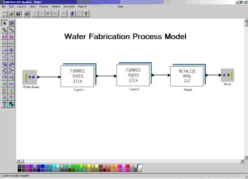
In fact, Simprocess is based on the description of graphical processes that describe the model’s behavior.
The following are the main characteristics of Simprocess:
- It is a hierarchical, event-oriented simulation tool.
- It can generate cost reports.
- Its simulations are based on activities, not machines.
- It uses templates.
- It uses additional logic (if, then, else).
- It considers and completely defines resources and can use fractional resources.
- Due to its hierarchical structure, each process can have an operation named process that defines a complete process, which enables the hierarchical definition of complete processes.
This can be done in a similar way in Arena®, which is very similar to Simprocess® (Figure 1).
 |
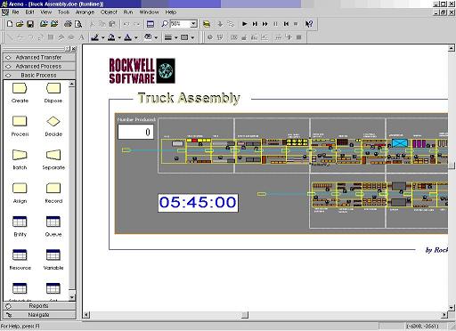 |
Figure 1. Simprocess and Arena(r) models.
This hierarchical process-definition tool can use templates, generate complete reports, etc.
An Arena’s important feature is that its models can be very similar to the real world (using DLLs inside simulation models and Visual Basic for Applications® allowing the use of specialized code). This makes Arena a powerful simulation package, because if the process-interaction paradigm cannot represent reality, all of the particularities can be programmed in VB or with an external DLL.
A DLL can also recover some information from the simulation model and send it, via TCP/IP, to a receiver that acquires and processes it[1]. This can be useful for constructing training systems (Fonseca, Casanovas et al. 2004). Figure 3 shows an example of an Arena model.
These packages use the process-interaction paradigm to describe the models. Other software programs, however, do not follow this paradigm, such as Witness®. This software follows a special paradigm (Witness 1998) (Figure 2). In fact, this software constructs processes using push/pull rules in the different model elements.
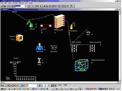
Figure 2. Witness model.
This methodology justifies the need for elements (which represent the real machines of the system) in simulation models, whereas Simprocess, Arena, GPSS and others only have operations. This is useful for representing more realistic models. However, if the Witness elements cannot fully represent the complexity of the system’s elements, problems can arise. To overcome this obstacle, Witness includes process definitions inside the entities. In this case, elements do not represent machines from the real world but rather operations, like in Arena and Simprocess.
Witness allows if…then…else rules to be defined in its push/pull rules[2], which allows entity routes to be modified. The different entities and resources[3] in Witness have attributes, but the model cannot easily modify these attributes, due to the limitations of this simulation language.
Artificial intelligence simulation software
Artificial intelligence (AI) simulation models are usually based on multi-agent systems (MAS). One of the most appealing approaches is Swarm, a set of libraries created by the Santa Fe Institute[4], which is designed to support complex simulation models.

Figure 3. Swarm logo.
The nucleus of a Swarm-based simulation is the model itself. Unlike other methodologies, the model has no external structures (in an event-scheduling simulation engine, the nucleus basically consists of a simulation loop and an event list, which are not a part of the model). In a simple case, the model is a structure named Swarm, occupied by a set of agents and a chronology of the activities that the agents will perform. Each agent is an object, created by the Swarm libraries and specialized through an inheritance mechanism.
In Swarm, the simulation-model construction process has a common set of tasks, but since each set of agents “lives” in a different environment, this is not a universal process.
In a Swarm simulation, the environment can also be modeled using an agent. The simulation kernel can therefore be reduced to the Swarm environment. For instance, in a simulation representing the evolution of a certain predator and its prey, the agent that represents the environment can also represent the growth of the vegetables that the prey eats.
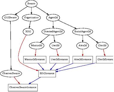
Figure 4. Swarm model structure example.
Obviously, this agent has a special status in the simulation model, but in the program parameters this agent is treated just like any other.
In fact, in the general case, the environment used by the agents consists of the agents themselves. This means that no specific agents are created to describe the behavior of the model. Some agents have more influence over the model than others, but the system manages all agents equally.
Once the user has defined the agents and their relationships, all of the agents are added to the Swarm system. The user writes a chronograph of activities for each agent and defines how time is simulated in the system. The set of actions is performed by the agent in the specified order.
These chronographs are created by using the instances of the structures of the Swarm library to fill the object/message structures. Once the chronograph is set, the Swarm model is ready to run.
|
Agent name:
|
Description:
|
|
Agent2D
|
Represents agents in a 2D world.
|
|
DirectAgent2D
|
Moves in a specified direction.
|
|
User2D
|
Follows other agents.
|
|
Marcus2D
|
Two behaviors:
When the agent has consumed all of its energy resisting, it enters an incubation period.
|
|
SocialAgent2D
|
Has strong relationships.
|
|
Alex2D
|
Follows the state of other agents.
Adds observations to its state.
|
|
Glen2D
|
Implements the following algorithm:
|
Table1. Swarm agents.
Table 1 details the most important Swarm agents and Figure 4.9 shows a Swarm model structure.
A Swarm model is of no interest if no data can be acquired by running it. According to the Swarm philosophy, a system has a set of agents that can acquire data: the observers.
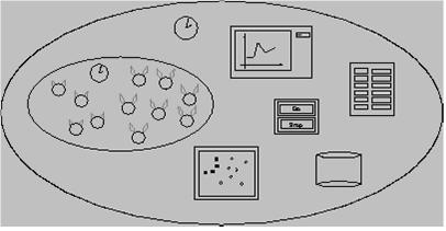
Figure 5. Swarm observer.
For instance, an observer agent (Figure 6) can see the number of prey and show the evolution of the population in real time using graphics. Other agents can analyze the spatial distribution of the predators.
Observer agents are Swarm agents like all the others, but their chronographs focus on acquiring data from the model. In fact, Swarm is a set of protocols that can describe the behavior of objects (objects named agents that experiment with space and time).
Another interesting system is Framsticks (Komosinski and Szymon 2000). This system tests the evolutionary capacity of creatures designed by the modeler. The environmental conditions are usually similar to earth conditions. The system works in a three-dimensional environment and allows the physical structures of the creatures to relate to the environment.
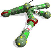 |
Name: Owohyw Ris Genotype: rrCCii(rXX[| T :379.564],r(rXX[@ 0 :-3.182][| G :1.749],X[| 0 :-135.911,G :0.878]),X) Average horizontal speed: 0.002 |
Figure 6. Framsticks agent.
Organisms are described by genomes and a neuronal network communicates with the environment. This network also processes the signals that come from the environment and implements behavior.
The creatures have energy needs and the notion of energy efficiency. As a result, they develop survival mechanisms: they passively take energy from the environment and, more aggressively, they kill other creatures to take their energy. The simulator allows the user to see the creatures’ evolution. Specifically, it allows the user to study the evolution of the creatures’ movement mechanisms and their ability to find energy, avoid predators and catch prey. From the definition of the initial creature characteristics, complex behaviors can emerge – behaviors that can be analyzed and studied. Also its representation determines their movement capacity and hence their survival effectiveness.
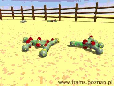 |
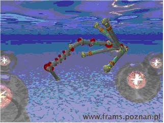 |
Figure 7. Two Framsticks structures.
These two systems create a global behavior (emergence). Swarm works with multiple intelligent agents that have defined behavior. From their actions, an emergent behavior appears. These agents usually do not have equivalence in the empirical real world and are usually too abstract to make social sense (Werner 2000). This sometimes makes the task of redefining agent behavior impossible (because it is difficult to completely define the behavior of some individuals). Framsticks works with creatures that implement a network. Framsticks worlds usually do not have equivalence in the real world. Its utility lies in the ability to analyze the characteristics of the different elements.
Other systems are MASON, RePast, AgentSheets. MASON is a single-process discrete-event simulation core and visualization toolkit written in Java, designed to be flexible enough to be used for a wide range of simulations, but with a special emphasis on “swarm” simulations of a very many (up to millions of) agents. The system is open-source and free, and is a joint effort of George Mason University’s Computer Science Department and the George Mason University Center for Social Complexity. MASON may be downloaded at http://cs.gmu.edu/eclab/projects/mason/ (Luke, Cioffi-Revilla et Alt. 2004).
Repast are in alpha stage of development, while AgentSheets is commercial software that allows the definition of different agents that interact together.
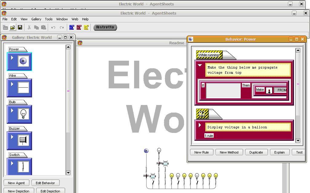
Figure 8. AgentSheets environment.
In the previous figure, the AgentSheets environment is shown
Simulation programming libraries and infrastructures
From the DEVS formalism, we can define simulation languages by using the specification paradigm to directly construct the model.
DEVSJAVA uses Java to construct simulation models following the DEVS formalism. This system is based on the DEVS formalism and does not have a specific scope; hence, we can model any kind of system. For more information about DEVSJAVA, see Zeigler and Sarjoughian (2003).
Another standard infrastructure, High Level Architecture (HLA), can create simulations made up of different software components.
Complex simulations usually involve a combination of various elements that have different objectives and structures. As a result, these components must often be modified in order to use them in the model. Hence, it is sometimes easier to implement a new system. In fact, traditional simulation models are not reusable or interoperable in different scenarios and applications.
Interoperability is related to reusability. Interoperability means that reusable components can be combined without modifying the code.
Interoperability includes the ability to combine different simulation components, sometimes with operations that take place in real time. This approach involves considering how simulation components interact in a traditional simulation program. Rather than developing a simple program running on an isolated computer, we need to develop a set of programs that can run together on multiple computers of different types that interact with each other in a real-time environment. For instance, to create a training model for the nuclear industry, different simulation models need to be developed. Some can represent the movement of the different elements in the factory; others can represent real-time elements that the user frequently modifies while the model is running. A standard must therefore be developed to interconnect these elements. To solve this problem, an area of the DoD called the Defense Modeling and Simulation Office (DMSO) developed HLA. Its main purpose was to support the needs of Army-related projects. It is now widely used in many other areas. The DoD shares HLA information inside and outside the US, helps new users evaluate and implement simulation infrastructures and reduces complexity and costs with tools and documentation. Applications outside the DoD include traffic and industrial simulations.
In HLA, a simulation model is a hierarchy of components with an increasing level of aggregation. The lower level may contain the model of a system component, a mathematical model, a queue model or a rule-based model. The model is implemented using software that produces the simulation. Simulations carried out as a part of an HLA simulation model are called federates. In HLA, simulations that include a number of federates are called federations. Various instances of a specific federate can exist, which means that HLA simulation models are modular. Federations can include much more than just simulations, such as human interfaces to assist the interaction with machines in real time, data analyzers, etc.
Summary
The following table (Table 2) presents the major features of the simulation models described above and others.
The user column summarizes the programming knowledge needed to use the system. Level 3 indicates high programming knowledge, while Level 0 indicates that the user does not need any programming knowledge.
The Source column shows if the source is available for its modification without restrictions.
The interface columns shows the way the user interact with the application.
|
Name
|
Language
|
Interface
|
Goal
|
Source
|
Version
|
User
|
|
|
Framsticks
|
N/A
|
Software
|
MAS
|
No
|
V 2.11
|
1
|
|
|
Swarm
|
Objective C, Java
|
Libraries
|
MAS
|
Yes
|
|
3
|
|
|
Arena
|
Visual Basic
|
Software
|
Discrete event simulation
|
No
|
V 8
|
0-3
|
|
|
Witness
|
Proprietary language
|
Software
|
Discrete event simulation
|
No
|
V 2006
|
0-2
|
|
|
LeanSim
|
C++
|
Software, Libraries
|
Discrete event simulation, training systems construction
|
Yes
|
V 1.0
|
0-3
|
|
|
SLAM
|
Proprietary language
|
Text editor
|
Discrete event simulation
|
No
|
V 4.2
|
1
|
|
|
GPSS/H
|
GPSS
|
Text editor
|
Discrete event simulation
|
No
|
V 4.3.5
|
1
|
|
|
Vensim PLE
|
N/A
|
Software
|
Continuous simulation
|
No
|
V 5.5d
|
0
|
|
|
MASON
|
Java
|
Libraries
|
MAS
|
Yes
|
V 11
|
3
|
|
|
Repast
|
Java
|
Libraries
|
MAS
|
Yes
|
Alpha
|
3
|
|
|
AgentSheets
|
N/A
|
Software
|
MAS
|
No
|
V 2.5
|
0
|
|
Table 2: Analyzed simulation systems.
[1] An application of this type was developed in the LCFIB to analyze, in real time, a set of systems that control the AGV fleet of a major food company. A communication library made it possible for the model (constructed with Arena) to receive external information through TCP/IP. This communication allows the overall system to be debugged without the problems that would be created by a real experiment.
[2] The TO rule of a Witness element can define the direction of an entity. With this rule, we can define if…then…else rules using all elements of the model (“if atr=1 then PUSH machine(1) else PUSH machine(2) endif”). With these rules, the entity path can easily be modified using entity attributes or model attributes.
[3] In Witness, resources are the elements needed to perform an operation in a specific element (machine).
[4] Santa Fe Institute, 1399 Hyde Park Road, Santa Fe, New Mexico, 87501, USA.
[5] Computing Laboratory of the Barcelona School of Informatics.
References:
Fonseca i Casas, Pau; Casanovas, Josep; Montero, Jordi. 2004d. LeanSim® virtual reality distributed simulation suite. Proceedings of MSO 2004.
Komosinski, Maciej; Ulatowski, Szymon. 2000. Framsticks. In: Kybernetes: The International Journal of Systems & Cybernetics, Vol. 29, No. 9/10.
Pritsker, A. 1986. Introduction to simulation and SLAM II. Halsted Press.
Werner, Roland. 2000. Structure, flow, change: Towards a social systems simulation methodology. Social Systems Simulation Group. San Diego State University. Witness. 1998. User’s Manual, Version 9. Lanner Group.
Zeigler, Bernard P.; Sarjoughian, Hessam S. 2003. Introduction to DEVS modeling and simulation with Java: Developing component-based simulation models. Resources http://www.acims.arizona.edu/EDUCATION/education.shtml (accessed 17 January 2005).
GPSS
GPSS
Pau Fonseca i Casas; pau@fib.upc.edu
GPSS
General Purpose Simulation System. Developed by Geoffrey Gordon during 60‟s of XX century. Discrete systems modeling.
GPSS/H
GPSS world
Entities (transactions) traveling through the system. Through the blocs.
The
number of blocs is different depending on the GPSS version used.
GPSS/H
Architecture
Based in blocs diagrams. Blocs joined using lines representing a transactions sets, that makes its movement through the blocs. Entities making its path through the system elements. Transactions. Its movement is from bloc to bloc representing actions or events that affects the entities.
GPSS/H
Transactions
Temporal or permanent.
Temporal:
created and destroyed. Permanents: dynamic.
Have attributes. Individual and unique identifier.
GPSS/H
Files:
GPSS/H version:
.gps
(containing the model) .lis (containing the results of the model execution)
GPSS/H
Language structure
4 kind of instructions
1. 2. 3. 4.
System access instructions Variable definition instructions Program logic instructions Simulation control instructions
GPSS/H
System access instructions
GPSSH [file.gps] TV.
To
obtain the simulation control. Display. Trap: breakpoints. Set:
TV
off All the screen for the dialog window. TV on Shows the 3 windows.
GPSS/H
Display
PF Function keys. Blo Actual and total blocs. CEC Current event chain. ClocksAbsolut and relative clock. FEC Future event chain. Xact=“id” Features of the current transaction.
GPSS/H
Trap
Trap ScanBreakpoint in the start of the Scan Phase. Untrap Scan To delete the breakpoint.
GPSS/H
Variable definition instructions
Functions definition (FUNCTION) Machine number definition (STORAGE) Matrix definition (MATRIX) Numerical assignation of variables (EQU) Variable initialization (INITIAL) Histogram definition (TABLE) Operations definition (VARIABLE i FVARIABLE)
GPSS/H
Program logic instructions
Named blocs.
GPSS/H
Simulation control instructions
START END SIMULATE
GPSS/H
GPSS code example
SIMULATE * * ONE-LINE, SINGLE-SERVER QUEUEING MODEL * GENERATE 18,6 ARRIVALS EVERY 18 +- 6 MINUTES ADVANCE 0.5 HANG UP COAT SEIZE JOE CAPTURE THE BARBER ADVANCE 15,3 HAIRCUT TAKES 15 +- 3 MINUTES RELEASE JOE FREE THE BARBER TERMINATE 1 EXIT THE SHOP * START 100 END
GPSS/H
Blocs (I)
Permanent and static entities (do not flow through the model). Used by transactions to do some jobs.
Facilities
(1). Storages (n).
GPSS/H
Blocs (II)
Describing how the entity flows throw the model. Representing action or event. Combination of blocs process defining what happens to a transaction model logic. Graphical representation.
Clear explanation. Helps in the design.
GPSS/H
Entity (Transaction on GPSS)
Destination route. Related statistics.
Blocs
visited. Waiting time.
Kind.
GPSS/H
Simulation object
State Number of elements in the queue. Related statistics. Kind of object.
GPSS/H
Event
Creation time. Execution time. Priority Kind of event.
Depending
on the kind of event a simulation element develops one action or other.
GPSS/H
Modification in the state of a simulation element.
GPSS/H
Blocs
Program logic instructions
GPSS/H
Generate
Creation of model transactions. Time between arrivals: random variable. A: Average interval time. B: ½ range (A ± B). C: Time for the first transaction. D: Maximum number of created transactions. E: Priority level F: Number of parameters.
GPSS/H
Terminate
To destroy the transactions. A: Number to decrement the TC.
GPSS/H
Advance
Stops the transaction movement some time. A: Average waiting time B: ½ range
GPSS/H
Example
Museum
GPSS/H
Modeling simple servers
People or objects that performs a service. Limited resourceKind:
1 server by time unit. Complex more than one server by time unit.
Simple
GPSS/H
Seize
The entity request the server. A: Identifier of the requested server.
GPSS/H
Release
To release a server. A: Identifier of the released server.
GPSS/H
Example: Manual lathe
A manual lathe process wooden pieces with a 5±2 minutes (uniform distribution). The arrival of the pieces follows a uniform distribution of parameters 7±3 minutes. Develop a GPSS model to simulate the process of 500 pieces. Pieces arrival: 7±3 (uniform, minutes) Time to process a piece: 5±2 (uniform, minutes).
GPSS/H
Example: Manual lathe (answer)
GENERATE 7,3 SEIZE TORN ADVANCE 5,2 RELEASE TORN TERMINATE 1
Modeling complex servers
Is needed to define the server capacity. STORAGE S(ASCENSOR),6 Is needed to show when the server is requested and when the server is released.
GPSS/H
Enter
Request of one ore more parallel servers. Simulates the enter of the entity in the server. A: server‟s name. B: number of servers requested.
GPSS/H
Leave
To simulate the release of one or more servers. A: server‟s name. B: number of servers to release.
GPSS/H
Queue
To model the queues in front of a server.
A:
queue identifier. B: number of elements entering in the queue. Optional, 1 by default.
GPSS/H
Depart
To show that an entity is leaving a queue.
A:
queue identifier. B: number of elements leaving the queue. Optional, 1 by default.
GPSS/H
Queue Reports (I)
Queue: queue identifier. Max Count: queue maximum contents. Avg count: queue average contents. Total entries: queue total entries.
GPSS/H
Queue Reports (II)
Zero entries: entries with delay time = 0. Percent Zeros: % of entries that are zero entries. Avg Time: average time of stay in the queue. $Avg Time: average time without the zero entries.
GPSS/H
Example: Banc Fortuna v1.0
In a banc the clients arrives following a uniform distribution of 5 to 9 minutes. 1 single cashier. Service time of 2 a 6 minutes, following a uniform distribution. Simulate 500 clients.
GPSS/H
Example: Banc Fortuna v1.0 (answer)
GENERATE QUEUE SEIZE DEPART ADVANCE RELEASE TERMINATE
7,2 CUA CAIXER CUA 4,2 CAIXER 1
GPSS/H
Example: Banc Fortuna v1.1 (answer)
GENERATE QUEUE SEIZE ADVANCE RELEASE DEPART TERMINATE
7,2 COLA CAIXER 4,2 CAIXER COLA 1
Assign
Allows the modification of the transaction parameters. A: parameter‟s number. B: value to assign. C: kind of the parameter.
1. 2. 3. 4.
PHhalf word. PFfull word. PLfloating point. PBbyte.
GPSS/H
Labels
Is allowed to name the GPSS blocs.
To
access the SNA‟s. To break the transaction sequence.
GPSS/H
SNA‟s
Some information related to the model entities. Can be used in simulation time. Give information about the simulated model. Examples:
C1: Clock N$label : #Xacts
GPSS/H
Test
Allows compare values and control the destination of a transaction. X: relation operator. A: verification operator. B: Reference value. C: number of the destination bloc.
GPSS/H
Test
If the operand C is not defined, TEST is working in conditional mode. The transaction enters in the bloc and, when the condition is true, continues its movement. If C is specified, when the condition if false the transaction jumps to C. Values for X:
E: equal G: bigger GE: bigger or equal. L: les LE: les or equal. NE: no equal.
GPSS/H
Example: Banc Fortuna V3.0
In a banc the clients arrive following an uniform distribution with parameters 5 to 10 (minutes). 3 tellers. Service time: 2 to 5 minutes (uniform distribution). Simulate 1 day of work. At the end of the day no client must remain in the banc.
GPSS/H
Example: Banc Fortuna V3.0 (answer)
SIMULATE STORAGE GENERATE TEST LE ENT QUEUE FILA ENTER DEPART ADVANCE SORT LEAVE FIN TERMINATE S(CAIXES),3 7.5,2.5 C1,240,FIN CAIXES FILA 3.5,1.5 CAIXES
* *Blocs de control de terminació * GENERATE 240 TEST E N(ENT),N(SORT) TERMINATE 1 START 1 END
GPSS/H
Transfer
Allows to break the sequential movement of a transaction.
Transfer
A:tranference modality
Both,
All, Pick, FN, P, SBR, SIM, Fraction, Number, SNA,
Null
Optional parameter.
GPSS/H
Transfer
B: number or bloc position. C: number or bloc position. D: number or bloc position.
GPSS/H
Transfer
TRANSFER .40,OPC1,OPC2 TRANSFER BOTH, SEC1,SEC2 TRANSFER ALL,EJE1,EJE3,4 TRANSFER PICK,PRIMERO,ULTIMO TRANSFER FN,LUGAR,3 TRANSFER P,LUGAR,2 TRANSFER SBR,REG,MARC TRANSFER SIM,NORET,RET
GPSS/H
Example: TalsaV1.0
Two automatic lathes. Arrivals (4±1 uniform). Lathe A: 1 a 10 minutes (uniform). Lathe B: 2 a 15 minutes (uniform). Pieces enters in the first free, (we prefer the A). Simulate 50 pieces.
GPSS/H
Example: TalsaV1.0 (answer)
SIMULATE GENERATE QUEUE TRANSFER UNO SEIZE DEPART ADVANCE RELEASE 4,1 MATERIAL BOTH,UNO,DOS TALAD1 MATERIAL 5.5,4.5 TALAD1
TRANSFER
DOSSEIZE DEPART ADVANCE RELEASE PROD TERMINATE START END
,PROD TALAD2
MATERIAL 8.5,6.5 TALAD2 1 50
GPSS/H
FUNCTION
Allows to define a new probability distribution. Name FUNCTION A,B
X1,Y1/X2,Y2/../Xn,Yn
GPSS/H
FUNCTION
Nom: Reference name of the function. A: Function arguments. B: Type of the function.
(C,D,E,L,M).
Xi,Yi: Pair of data to create the distribution function.
Xi reference value. Yi is the value that the function returns.
GPSS/H
FUNCTION C
Continuous.
Given
an X value, interpolates and returns a value for
Y. As an example:
A=RN1 The
function must be defined between 0 and 1.
GPSS/H
FUNCTION D
Discrete. Growing values of X. If we find a value equals or greater than X we return its related value. If we do not find this value, returns the greater value.
GPSS/H
FUNCTION E
Discrete function of attribute value.
Returns
for an X the attribute value. RESUL FUNCTION X$VALOR,E3
1,S$ALM1/5,S$ALM2/9,S$ALM3
GPSS/H
FUNCTION L
Value list Returns the value of the X position (argument) TIPUS FUNCTION P2,L4
1,3/2,5/3,8/4,12
GPSS/H
FUNCTION M
Attribute value list Returns the value of the attribute in the position X (argument) LLISTA FUNCTION X$NOM,M3
1,X$NOM1/2,X$NOM2/3,X$NOM3
GPSS/H
Functions important aspects
1. 2. 3. 4.
Functions C,D,L do not admit SNA‟s ans Y‟s. Functions E, M must have SNA‟s as Y values. Functions L and M cannot use random arguments. To use a function:
1. 2.
FN(nom). F$nom(parametres).
GPSS/H
Example: Wooden tool v1.0
Arrivals 5 a 9 minutes (Uniform) Tool service time (minutes)
1
.4
Temps de procés
Freqüència relativa
2
3
4
5
.3 .15 .10 .05
Model this system during 8 hours.
GPSS/H
Resposta Serreria V1.0
SIMULATE TRAB FUNCTION RN1,D5 .4,1/.7,2/.85,3/.95,4/1,5 GENERATE 7,2 QUEUE UNO SEIZE MAQ DEPART UNO ADVANCE RELEASE MAQ TERMINATE * *Blocs de control de terminació * GENERATE 480 TERMINATE 1 START 1 END
FN(TRAB)
GPSS/H
Logic
Allows the modification of the logic bloc that represents.
X:
Logic operator.
S
(set) R (reset) By default I (Invert)
A:
logic control identifier.
Gate (1/2)
Controls the transaction flow. A: name or number of the analyzed installation. B: name of the label. X: Auxiliary operator. GATE NU INST,ALT
GPSS/H
Gate (2/2)
Related to SEIZE i RELEASE
U Try if the installation is full. NU Try if the installation is free. SF: Try if the server is full. SNF: Try if the server is not full. SE: Try if the server is empty. SNE: Try if the server is not empty. LS: Set logic LR: Reset logic.
Related to ENTER i LEAVE
Related to LOGIC
GPSS/H
Example: ViatgesV1.0
The clients call the travel agency following an uniform distribution (3±2 minutes). Give the information to the clients follows an uniform distribution of 5 to 8 minutes. If the telephone is occupied the client is lost. Simulate 8 hours.
GPSS/H
Example: ViatgesV1.0 (answer)
SIMULATE GENERATE GATE NU SEIZE ADVANCE RELEASE OTRO GENERATE TERMINATE START END
GPSS/H
3,2 TELEF,OTRO TELEF 6.5,1.5 TELEF
TERMINATE 480 1 1
Savevalue
To give or modify the value of a SAVEVALUE element. A: SAVEVALUE name. B: Value assigned to the SAVEVALUE (integer, name or SNA). C: SAVEVALUE type:
XH half word. XF full word. XL floating point. XB byte.
GPSS/H
Accessing to a SAVEVALUE
We can access the value stored in a SAVEVALUE in any part of the GPSS program through the sentence:
X(nom)
(XH, XF, XL, XB) [H] X$nom [W]
GPSS/H
Matrix
Name MATRIX A: Matrix type. B: Files. C: Columns.
MAGATZEM
A,B,C
MATRIX MH,200,4 Defines a 200 x 4 matrix.
GPSS/H
Msavevalue
To give or modify the value of a matrix. A: name. B: file number. C: column number. D: information to be stored.
GPSS/H
Initial
To initialize the LOGICSWITCH, SAVEVALUE or the matrix. INITIAL LS5,1. INITIAL XH(1),10. INITIAL XF(1),10. INITIAL XL(1),10. INITIAL XB(1),10. INITIAL MX$nom(1,2),5.
GPSS/H
Ampervariables (definició)
Global varialbes INTEGER &I,&D(10) REAL &Pes CHAR*10 &C VCHAR*4 &Títol
GPSS/H
Ampervariables (Initialization)
LET.
LET &var=A.
GETLIST &var1,&var2.
GETLIST.
The user interacts with the model adding some information.
Can be used as a blocs.
BLET. BGETLIST.
GPSS/H
Loop
Allows to modify the destination of an active transaction. A: Parameter containing the number of times a transaction passes an specific section. B: Destination.
Example: Loop
REG
ASSIGN voltes,10 ENTER SERV .. LOOPvoltes,REG SEIZE CAJERO
GPSS/H
Example: Wagons V1.0
5 transport wagons (of pieces) between two points. Initial point: loaded by 1 worker with 50 pieces. U(5,7) seconds x piece. Movement to the final point U(4,8) minutes. Download by a second worker. U(10,16) seconds x piece. Movement to the origin U(3,7) minutes. Simulate 24 hours.
GPSS/H
Example: Vagons V1.0 (answer)
GENERATE ,,,5 CICLE ASSIGN QUEUE SEIZE MAS LOOP RELEASE DEPART ADVANCE ASSIGN QUEUE SEIZE MEN CARB,50 INI CARG ADVANCE CARB,MAS CARG INI 360,120 CARB,50 FIN DESC ADVANCE 13,3 6,1 START END 1 GENERATE TERMINATE 86400 1
LOOP
RELEASE DEPART ADVANCE TRANSFER
CARB,MEN
DESC FIN 300,120 ,CICLE GPSS/H
Split
Allows the creation of new transactions with the same features of active transaction. A: Nº of new created transactions. B: Destination of the new transactions (op). C: Parameter that receives the serial number.
GPSS/H
Example: TaladreSplit V1.0
Entities every 8 hours. Size of the lotes:
Lot size Probability 17 18 19 20 21
0.1 0.4 0.4 0.05 0.05
Service time 10±5 Simute 3000 pieces
GPSS/H
Example: TaladreSplit V1.0 (sample)
LOT FUNCTION RN1,D5 .1,16/.5,17/.9,18/.95,19/1,20 SIMULATE * * * ONE-LINE, SINGLE-SERVER QUEUEING MODEL GENERATE SPLIT 480 FN$LOT,TAL
TAL QUEUE SEIZE
DEPART ADVANCE RELEASE TERMINATE * START END
ALM TALAD
ALM 10,5 TALAD 1 3000
GPSS/H
Funavail
Allows that an installation be available. A: name of the instalation. B: Modality. (op)
RE: remover. CO: Continuar. Nul.
C: name of the bloc for the transaction that owns the instalation. (op)
Funavail
D: number of the parameter that receives the residual time if the transaction is expulsed from the installation. (op) E: Modality de RE o Co. (op) F: name of the bloc for the PREEMP transactions of the instalation. (op)
GPSS/H
Funavail
G: Modality RE o CO for the delayed transactions. (op) H: name of the new bloc for the pending transactions of the installation. (op)
GPSS/H
Favail
Assures that an installation must be available. A: name of the installation
GPSS/H
Sunavail
Assure that the STORAGE is not available. A: STORAGE name.
GPSS/H
Savail
To guarantee that the STORAGE is available. A: STORAGE name.
GPSS/H
Maquinat example
New work every 10±4 minutes. Working time 15±5 minutes. Every 90 minutes both 2 machines stops during 15 ±3 minutes. Simulate 1000 pieces.
GPSS/H
Maquinat answer
STORAGE SIMULATE GENERATE QUEUE ENTER DEPART ADVANCE LEAVE 10,4 INV MAQ INV 15,3 MAQ S(MAQ),2
TERMINATE
GENERATE SUNAVAILMAQ ADVANCE SAVAIL TERMINATE START END
1
90 15,3 MAQ
1000
GPSS/H
Trace
Starts the trace of the transactions properties. The information that are printed are:
Number
of the transaction. Current block. Destination block. Clock value.
GPSS/H
Untrace
Stops the trace of the transaction properties.
GPSS/H
Assemble
To synchronize transactions. A: Number of transactions we are looking for.
GPSS/H
Gather
To synchronize transactions. A: number of transactions we are waiting for.
GPSS/H
Match
To synchronize transactions. A: The other block MATCH.
GPSS/H
Lathe example
Pieces every 6 minutes. One worker, 3 phases of work.
1. 2. 3.
Lathe 3 minutes for piece. Take piece new dimensions (no time. Rectification 2 minutes piece.
Recalibration of the machine that takes the dimensions for each piece 5±3 minutes done by other worker. On the rectification the machine must be recalibrated. Simulate 200 pieces.
GPSS/H
Tornejat answer
SIMULATE GENERATE 6
QUEUE
SEIZE DEPART SPLIT ADVANCE MED1 MATCH ADVANCE
ALM
OPER ALM 1,MED 3 MED2 2 Starts the calibration of the piece Working Wait for the calibration of the machine
RELEASE
TERMINATE MED MED2 ADVANCE MATCH TERMINATE 1
OPER
5,3 MED1
START
END
200
GPSS/H
Modify the position of the transaction on FEC and CEC
Modify the priority. Suspend the active transaction. Catch a machine, moving the transaction that owns it.
GPSS/H
Priority
Defines the priority over the active transaction. A: new priority value.. B: Buffer option. (op). (see BUFFER).
GPSS/H
Buffer
Allows to reanalyze the CEC.
GPSS/H
Preempt
Displaces the transaction that owns the installation allowing that the new transaction takes it. A: installation id. B: priority mode. (op). C: identifier of the bloc for the moved transaction. (op). D: number of the parameter that receives the residual time. (op).
GPSS/H
Preempt
E: Remover modality. (op)
GPSS/H
Return
Free an installation that was been captured by a transaction. A: Installation name.
GPSS/H
Replications (repetitions)
To analyze the model n DIFERENT experiments are required. Different behavior based on different RNG. To execute N different experiments. Between 3 an 10 replications. Calculus of the mean and the variance from these replications.
GPSS/H
Transitory period
Loading period of the model.
GPSS/H
Clocks GPSS/H
Relative clock: Time from the beginning of the simulation until the execution of RESET or CLEAR. Absolute Clock: Time from the beginning of simulation until the execution of CLEAR.
GPSS/H
Reset
RESET doe not delete the transactions of the current model. The blocs contents are not modified.
The statistic value total counts is set to current counts. (CLEAR put this to 0).
Relative clock to 0. RNG are not initialized. Usually to define the loading period.
GPSS/H
Clear
Deletes all the transactions. Current counts and total counts set to 0. Clocks to 0. All the servers are set to free. RNG are initialized.
GPSS/H
Clear
Blocs contents set to 0. LOGICS set to 0. MATRIX elements set to 0. SAVEVALUES set to 0.
GPSS/H
Transitory Time
Time discarded from the statistics acquisition.
GPSS/H
In/Out on GPSS/H
File definition FILEDEF (control instruction)
OUT1
FILEDEF
„Sortida.txt‟
Inside the model the reference to the file is based in OUT1.
GPSS/H
Getlist
GetList FILE=nom,END=A,ERR=B,(&var1,&var2,..). Nom: logic name for the file to read the info. A: label of the control instruction if EOF is found. B: label of the instruction when read error is found. &var1: variable list to be read.[req].
GPSS/H
Bputpic
To print the results. Name: name of the file. K: Number of text lines below the PUTPIC or BPUTPIC for the impressions of the results. A,B,C,..: Variable list, SNA, Savevalues, ampervariables to be printed.
PUTPIC FILE=SAL,LINES=2,(FC1,FC2). Num. pieces machine 1: ******. Num. pieces machine 2: ******.
GPSS/H
Uniform distribution
A,B AB Inter Arrival Time = (A-B) + RN1*(2*B). RN1 on GPSSH is transparent for the user.
GPSS/H
Distribució exponencial
RVEXPO(j,IATave) IATave= Temps mig entre arribades.
GPSS/H
Poisson and Exponential
Poisson nº of occurrences by interval. =30 arrivals/hour. Exponential Time between arrivals =1/30 hours=2 minutes.
GPSS/H
Erlang distribution
(,K)=k exponencials de mitja /K ADVANCE RVEXPO(3,0.45) ADVANCE RVEXPO(3,0.45) ERLANG(0.9,2) ADVANCE RVEXPO(3,0.45)+ RVEXPO(3,0.45)
GPSS/H
Normal distribution
RVNORM(j, , ) Be careful with the negative numbers ABS(RVNORM(j, , ))
GPSS/H
Triangular distribution
RVTRI(j,min,mode,max)
GPSS/H
Example of some distribucions
SIMULATE * * ONE-LINE, SINGLE-SERVER QUEUEING MODEL * GENERATE 1 ADVANCE 5,2 ADVANCE RVEXPO(3,0.45) ADVANCE RVEXPO(3,0.45)+RVEXPO(3,0.45) ADVANCE ABS(RVNORM(1,5,3)) ADVANCE RVTRI(1,2,3,5) TERMINATE 1 *
GPSS/H
Internal vision of the transactions movement
Understanding the process interaction paradigm
GPSS/H
Example (Blocs)
1. 2. 3. 4.
5.
6. 7.
Entering 3 ± 1 minutes Start Storage Entering Resource Exit Storage Using the resource 3 Release resource Exit system
GPSS/H
Example (Programming blocs)
1.
New entities arrivals
3 ± 1 minutes
2. 3.
Verification and capture of the free resource Using the resource
3 minutes
4. 5.
Release the resource The entity leaves the system
GPSS/H
Exemple (+ presa de estadístiques)
1.
New entities arrival
3 ± 1 minutes
2. 3. 4. 5.
Inici de la presa de estadístiques de la possible acumulació. Verificació i captura del torn desocupat Fi de la presa de estadístiques de la possible acumulació Tornejat de la matèria prima
3 minuts
6. 7.
Alliberar el torn Sortida del producte del sistema
GPSS/H
Exemple (Cadenes d‟esdeveniments)
1.
Entrada de una transacció i en el sistema.
En t també entra la peça i+1 a la cadena d‟esdeveniments futurs, en la que estarà fins t+u(2,4). Si la peça entra passarà al següent bloc seqüencial. Si el torn està ocupat la transacció s‟envia a la part final de la cadena d‟esdeveniments actuals, en la que romandrà fins que el torn quedi lliure.
2.
1. 2.
Verificació de la entrada en el torn.
3.
4.
5.
Entrada en la cadena d‟esdeveniments futurs on estarà 3 minuts. Sortida de la cadena d‟esdeveniments futurs i alliberació del torn. Sortida del sistema de la transacció.
GPSS/H
Programa en GPSS/H (punts de vista)
Visió externa de les transaccions. Punt de vista de programació en blocs.
Conjunt de blocs per els que flueixen les transaccions.
Visió interna de les transaccions. Punt de vista de les cadenes d‟esdeveniments.
Llocs on s‟envien les transaccions durant el seu recorregut a través del model o blocs que troben una condició de bloqueig que els impedeix de seguir el seu camí.
GPSS/H
Cadenes d‟esdeveniments (I)
Llista de transaccions. En qualsevol moment:
bloc. Transacció cadena.
Transacció
Quan una transacció es mou:
De
bloc a bloc. De cadena a cadena. De bloc a cadena. De cadena a bloc.
GPSS/H
Bloqueig en les Cadenes d‟esdeveniments
Bloqueig de retard:
La
transacció entra en un bloc en t1 i surt en t2.
algun motiu la transacció no por accedir al bloc.
Bloqueig condicional:
Per
GPSS/H
Tipus de cadenes
1. 2. 3. 4.
5.
Current esdeveniment chainsempre 1 Future esdeveniments chainsempre 1 Users chain0 o més. Interrupt chain0 o més. MAQ chains0 o més.
GPSS/H
Current event Chain (CEC)
Transaccions que es volen moure en el instant actual.
Poden
haver problemes que impedeixin que les transaccions no es moguin.
Bloquejats. Ocupats.
Ordenada
per prioritat decreixent.
GPSS/H
CEC
Move time: Current simulation time
GPSS/H
Future event Chain (FEC)
Les transaccions no intenten moure‟s en aquell moment, ha de passar un temps de simulació. Que ho provoca:
Entrar
en el model amb un GENERATE. La xact està en un bloc ADVANCE.
Ordenat per temps i prioritat.
GPSS/H
FEC
7,2,11 : blocs ADVANCE 9 : bloc GENERATE
GPSS/H
Exemple GPSS
GPSS World Simulation Report - TaladreSplit V1.0.3.1
Tuesday, March 08, 2005 10:40:14 START TIME 0.000 END TIME BLOCKS FACILITIES STORAGES 493.810 8 1 0
LABEL 1 2 3 4 5 6 7 8
TAL
LOC BLOCK TYPE GENERATE SPLIT QUEUE SEIZE DEPART ADVANCE RELEASE TERMINATE
ENTRY COUNT CURRENT COUNT RETRY 1 0 0 1 0 0 18 16 0 2 1 0 1 0 0 1 0 0 1 0 0 1 0 0
GPSS/H
Exemple GPSS
FACILITY TALAD ENTRIES UTIL. AVE. TIME AVAIL. OWNER PEND INTER RETRY DELAY 2 0.028 6.905 1 3 0 0 0 16
QUEUE ALM
MAX CONT. ENTRY ENTRY(0) AVE.CONT. AVE.TIME AVE.(-0) RETRY 17 17 18 1 0.475 13.043 13.810 0
CEC XN PRI 3 0
M1 ASSEM CURRENT NEXT PARAMETER 480.000 1 4 5
VALUE
FEC XN PRI 2 0
BDT ASSEM CURRENT NEXT PARAMETER 960.000 2 0 1
VALUE
GPSS/H
GENERATE blocs initialization
On time 0. In Top-Down order (GPSS/H) For each bloc one transaction are created. Identifiers are assigned consecutively. Assigning the moveTime for each transaction. If the moveTime is equals to 0, this transaction I queued in the CEC, otherwise in the FEC.
GPSS/H
Transactions movement
GPSS/H
SCAN PHASE
GPSS/H
UPDATE PHASE
GPSS/H
Exemple (Blocs)
1. 2. 3. 4.
5.
6. 7.
Entrada Inici Entrada Sortida Tornejat Sortida Sortida
3 ± 1 minuts Magatzem Torn Magatzem 3 Torn Sistema
GPSS/H
Exemple (dades)
Interval between generations:
(2,2,4,4)
We only generate 4 entities.
Temps Inici 0 CEC FEC (1,Fora,1,2) 1 2
Pas
GPSS/H
Example (event chains)
Step 1 2 3 4 Time Inici 0 2 2 CEC (1,Fora,1,Now) FEC (1,Fora,1,2) (2,Fora,1,4) (1,5,6,5) (1,5,6,5) (1,5,6,5) (3,Fora,1,8)
GPSS/H First Xact. Xact from FEC to CEC. Moving the Xact 1 all that we can, entering in 5 (advance). Generatio of the second Xact. Xact from FEC to CEC. Moving the Xact 2 all that we can, entering the 2 (seize). Generation of the third Xact.
Comments
5 6
4 4
(2,Fora,1,Now) (2,2,3,Now)
Example (event chains)
Step 7 8 Time 5 5 CEC (2,2,3,Ja) (1,5,6,Ja) FEC (3,Fora,1,8) (3,fora,1,8) (2,5,6,8) Comments
Xact from FEC to CEC.
Moving the Xact 1 all that we can, leaving the system. Moving the Xact 2 all that we can, entering the 5 (advance). Xact from FEC to CEC.
9
8
(3,Fora,1, Ja) (2,5,6,Ja) -
10
8
(3,5,6,11) (4,Fora,1,12)
Moving the Xact 2 all that we can, leaving the system. Moving the Xact 3 all that we can, entering the 5(advance). Programming the next arrival. GPSS/H
Example (event chains)
Step 11 12 13 14 15 16 Time 11 11 12 12 15 15 CEC (3,5,6,Now) (4,Fora,1,Now) (4,5,6,Now) FEC (4,Fora,1,12) (4,Fora,1,12) (4,5,6,15) Coments
Xact from FEC a CEC. Moving the Xact 3 all than we can, leaves the system. Xact from FEC a CEC. Moving the Xact 4 all that we can, entering the 5 bloc (advance). Xact from FEC to CEC. Moving the Xact 4 all that we can, leave the system.
GPSS/H