Simulation tools
Numerous computer programs can now be used for generic simulations. Each of these tools follows a different model-construction paradigm.
The major characteristics of certain simulation programs are described in the next four sections. The first section is devoted to classical OR simulation tools, which are based on the concept of process and/or push/pull rules. The second section describes tools that use artificial intelligence methods. The third section reviews certain programming libraries that can be used in model construction. Finally, the fourth section reviews the major features of the different programs and tools.
OR tools
OR encompasses a wide range of tools for specifying, constructing and running models.
These tools use different paradigms to represent the real world. The discrete-event paradigm includes classical languages such as GPSS/H® and Slam II® (Pritsker 1986). These tools have features similar to those of Simprocess® and Arena® and follow the process-interaction paradigm or the event-scheduling paradigm.
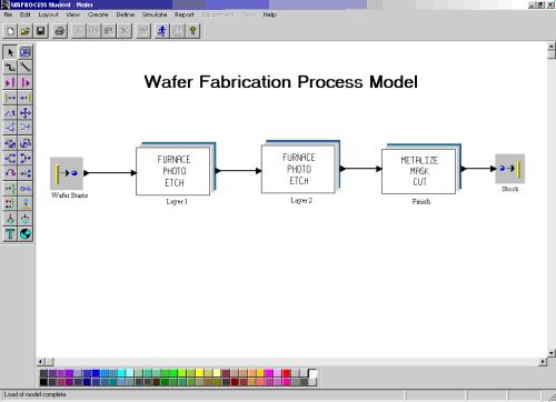
In fact, Simprocess is based on the description of graphical processes that describe the model’s behavior.
The following are the main characteristics of Simprocess:
- It is a hierarchical, event-oriented simulation tool.
- It can generate cost reports.
- Its simulations are based on activities, not machines.
- It uses templates.
- It uses additional logic (if, then, else).
- It considers and completely defines resources and can use fractional resources.
- Due to its hierarchical structure, each process can have an operation named process that defines a complete process, which enables the hierarchical definition of complete processes.
This can be done in a similar way in Arena®, which is very similar to Simprocess® (Figure 1).
 |
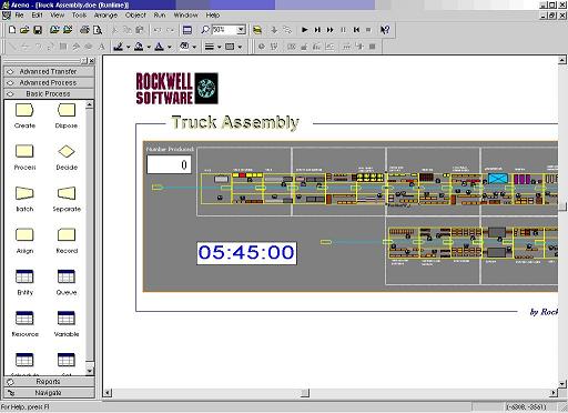 |
Figure 1. Simprocess and Arena(r) models.
This hierarchical process-definition tool can use templates, generate complete reports, etc.
An Arena’s important feature is that its models can be very similar to the real world (using DLLs inside simulation models and Visual Basic for Applications® allowing the use of specialized code). This makes Arena a powerful simulation package, because if the process-interaction paradigm cannot represent reality, all of the particularities can be programmed in VB or with an external DLL.
A DLL can also recover some information from the simulation model and send it, via TCP/IP, to a receiver that acquires and processes it[1]. This can be useful for constructing training systems (Fonseca, Casanovas et al. 2004). Figure 3 shows an example of an Arena model.
These packages use the process-interaction paradigm to describe the models. Other software programs, however, do not follow this paradigm, such as Witness®. This software follows a special paradigm (Witness 1998) (Figure 2). In fact, this software constructs processes using push/pull rules in the different model elements.
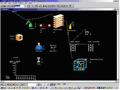
Figure 2. Witness model.
This methodology justifies the need for elements (which represent the real machines of the system) in simulation models, whereas Simprocess, Arena, GPSS and others only have operations. This is useful for representing more realistic models. However, if the Witness elements cannot fully represent the complexity of the system’s elements, problems can arise. To overcome this obstacle, Witness includes process definitions inside the entities. In this case, elements do not represent machines from the real world but rather operations, like in Arena and Simprocess.
Witness allows if…then…else rules to be defined in its push/pull rules[2], which allows entity routes to be modified. The different entities and resources[3] in Witness have attributes, but the model cannot easily modify these attributes, due to the limitations of this simulation language.
Artificial intelligence simulation software
Artificial intelligence (AI) simulation models are usually based on multi-agent systems (MAS). One of the most appealing approaches is Swarm, a set of libraries created by the Santa Fe Institute[4], which is designed to support complex simulation models.

Figure 3. Swarm logo.
The nucleus of a Swarm-based simulation is the model itself. Unlike other methodologies, the model has no external structures (in an event-scheduling simulation engine, the nucleus basically consists of a simulation loop and an event list, which are not a part of the model). In a simple case, the model is a structure named Swarm, occupied by a set of agents and a chronology of the activities that the agents will perform. Each agent is an object, created by the Swarm libraries and specialized through an inheritance mechanism.
In Swarm, the simulation-model construction process has a common set of tasks, but since each set of agents “lives” in a different environment, this is not a universal process.
In a Swarm simulation, the environment can also be modeled using an agent. The simulation kernel can therefore be reduced to the Swarm environment. For instance, in a simulation representing the evolution of a certain predator and its prey, the agent that represents the environment can also represent the growth of the vegetables that the prey eats.
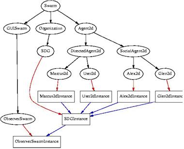
Figure 4. Swarm model structure example.
Obviously, this agent has a special status in the simulation model, but in the program parameters this agent is treated just like any other.
In fact, in the general case, the environment used by the agents consists of the agents themselves. This means that no specific agents are created to describe the behavior of the model. Some agents have more influence over the model than others, but the system manages all agents equally.
Once the user has defined the agents and their relationships, all of the agents are added to the Swarm system. The user writes a chronograph of activities for each agent and defines how time is simulated in the system. The set of actions is performed by the agent in the specified order.
These chronographs are created by using the instances of the structures of the Swarm library to fill the object/message structures. Once the chronograph is set, the Swarm model is ready to run.
|
Agent name:
|
Description:
|
|
Agent2D
|
Represents agents in a 2D world.
|
|
DirectAgent2D
|
Moves in a specified direction.
|
|
User2D
|
Follows other agents.
|
|
Marcus2D
|
Two behaviors:
When the agent has consumed all of its energy resisting, it enters an incubation period.
|
|
SocialAgent2D
|
Has strong relationships.
|
|
Alex2D
|
Follows the state of other agents.
Adds observations to its state.
|
|
Glen2D
|
Implements the following algorithm:
|
Table1. Swarm agents.
Table 1 details the most important Swarm agents and Figure 4.9 shows a Swarm model structure.
A Swarm model is of no interest if no data can be acquired by running it. According to the Swarm philosophy, a system has a set of agents that can acquire data: the observers.
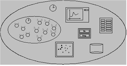
Figure 5. Swarm observer.
For instance, an observer agent (Figure 6) can see the number of prey and show the evolution of the population in real time using graphics. Other agents can analyze the spatial distribution of the predators.
Observer agents are Swarm agents like all the others, but their chronographs focus on acquiring data from the model. In fact, Swarm is a set of protocols that can describe the behavior of objects (objects named agents that experiment with space and time).
Another interesting system is Framsticks (Komosinski and Szymon 2000). This system tests the evolutionary capacity of creatures designed by the modeler. The environmental conditions are usually similar to earth conditions. The system works in a three-dimensional environment and allows the physical structures of the creatures to relate to the environment.
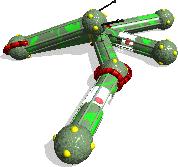 |
Name: Owohyw Ris Genotype: rrCCii(rXX[| T :379.564],r(rXX[@ 0 :-3.182][| G :1.749],X[| 0 :-135.911,G :0.878]),X) Average horizontal speed: 0.002 |
Figure 6. Framsticks agent.
Organisms are described by genomes and a neuronal network communicates with the environment. This network also processes the signals that come from the environment and implements behavior.
The creatures have energy needs and the notion of energy efficiency. As a result, they develop survival mechanisms: they passively take energy from the environment and, more aggressively, they kill other creatures to take their energy. The simulator allows the user to see the creatures’ evolution. Specifically, it allows the user to study the evolution of the creatures’ movement mechanisms and their ability to find energy, avoid predators and catch prey. From the definition of the initial creature characteristics, complex behaviors can emerge – behaviors that can be analyzed and studied. Also its representation determines their movement capacity and hence their survival effectiveness.
 |
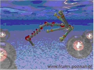 |
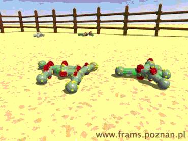
Figure 7. Two Framsticks structures.
These two systems create a global behavior (emergence). Swarm works with multiple intelligent agents that have defined behavior. From their actions, an emergent behavior appears. These agents usually do not have equivalence in the empirical real world and are usually too abstract to make social sense (Werner 2000). This sometimes makes the task of redefining agent behavior impossible (because it is difficult to completely define the behavior of some individuals). Framsticks works with creatures that implement a network. Framsticks worlds usually do not have equivalence in the real world. Its utility lies in the ability to analyze the characteristics of the different elements.
Other systems are MASON, RePast, AgentSheets. MASON is a single-process discrete-event simulation core and visualization toolkit written in Java, designed to be flexible enough to be used for a wide range of simulations, but with a special emphasis on “swarm” simulations of a very many (up to millions of) agents. The system is open-source and free, and is a joint effort of George Mason University’s Computer Science Department and the George Mason University Center for Social Complexity. MASON may be downloaded at http://cs.gmu.edu/eclab/projects/mason/ (Luke, Cioffi-Revilla et Alt. 2004).
Repast are in alpha stage of development, while AgentSheets is commercial software that allows the definition of different agents that interact together.
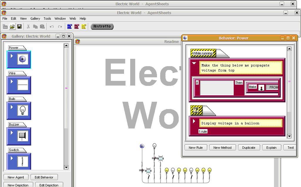
Figure 8. AgentSheets environment.
In the previous figure, the AgentSheets environment is shown
Simulation programming libraries and infrastructures
From the DEVS formalism, we can define simulation languages by using the specification paradigm to directly construct the model.
DEVSJAVA uses Java to construct simulation models following the DEVS formalism. This system is based on the DEVS formalism and does not have a specific scope; hence, we can model any kind of system. For more information about DEVSJAVA, see Zeigler and Sarjoughian (2003).
Another standard infrastructure, High Level Architecture (HLA), can create simulations made up of different software components.
Complex simulations usually involve a combination of various elements that have different objectives and structures. As a result, these components must often be modified in order to use them in the model. Hence, it is sometimes easier to implement a new system. In fact, traditional simulation models are not reusable or interoperable in different scenarios and applications.
Interoperability is related to reusability. Interoperability means that reusable components can be combined without modifying the code.
Interoperability includes the ability to combine different simulation components, sometimes with operations that take place in real time. This approach involves considering how simulation components interact in a traditional simulation program. Rather than developing a simple program running on an isolated computer, we need to develop a set of programs that can run together on multiple computers of different types that interact with each other in a real-time environment. For instance, to create a training model for the nuclear industry, different simulation models need to be developed. Some can represent the movement of the different elements in the factory; others can represent real-time elements that the user frequently modifies while the model is running. A standard must therefore be developed to interconnect these elements. To solve this problem, an area of the DoD called the Defense Modeling and Simulation Office (DMSO) developed HLA. Its main purpose was to support the needs of Army-related projects. It is now widely used in many other areas. The DoD shares HLA information inside and outside the US, helps new users evaluate and implement simulation infrastructures and reduces complexity and costs with tools and documentation. Applications outside the DoD include traffic and industrial simulations.
In HLA, a simulation model is a hierarchy of components with an increasing level of aggregation. The lower level may contain the model of a system component, a mathematical model, a queue model or a rule-based model. The model is implemented using software that produces the simulation. Simulations carried out as a part of an HLA simulation model are called federates. In HLA, simulations that include a number of federates are called federations. Various instances of a specific federate can exist, which means that HLA simulation models are modular. Federations can include much more than just simulations, such as human interfaces to assist the interaction with machines in real time, data analyzers, etc.
Summary
The following table (Table 2) presents the major features of the simulation models described above and others.
The user column summarizes the programming knowledge needed to use the system. Level 3 indicates high programming knowledge, while Level 0 indicates that the user does not need any programming knowledge.
The Source column shows if the source is available for its modification without restrictions.
The interface columns shows the way the user interact with the application.
|
Name
|
Language
|
Interface
|
Goal
|
Source
|
Version
|
User
|
|
|
Framsticks
|
N/A
|
Software
|
MAS
|
No
|
V 2.11
|
1
|
|
|
Swarm
|
Objective C, Java
|
Libraries
|
MAS
|
Yes
|
|
3
|
|
|
Arena
|
Visual Basic
|
Software
|
Discrete event simulation
|
No
|
V 8
|
0-3
|
|
|
Witness
|
Proprietary language
|
Software
|
Discrete event simulation
|
No
|
V 2006
|
0-2
|
|
|
LeanSim
|
C++
|
Software, Libraries
|
Discrete event simulation, training systems construction
|
Yes
|
V 1.0
|
0-3
|
|
|
SLAM
|
Proprietary language
|
Text editor
|
Discrete event simulation
|
No
|
V 4.2
|
1
|
|
|
GPSS/H
|
GPSS
|
Text editor
|
Discrete event simulation
|
No
|
V 4.3.5
|
1
|
|
|
Vensim PLE
|
N/A
|
Software
|
Continuous simulation
|
No
|
V 5.5d
|
0
|
|
|
MASON
|
Java
|
Libraries
|
MAS
|
Yes
|
V 11
|
3
|
|
|
Repast
|
Java
|
Libraries
|
MAS
|
Yes
|
Alpha
|
3
|
|
|
AgentSheets
|
N/A
|
Software
|
MAS
|
No
|
V 2.5
|
0
|
|
Table 2: Analyzed simulation systems.
[1] An application of this type was developed in the LCFIB to analyze, in real time, a set of systems that control the AGV fleet of a major food company. A communication library made it possible for the model (constructed with Arena) to receive external information through TCP/IP. This communication allows the overall system to be debugged without the problems that would be created by a real experiment.
[2] The TO rule of a Witness element can define the direction of an entity. With this rule, we can define if…then…else rules using all elements of the model (“if atr=1 then PUSH machine(1) else PUSH machine(2) endif”). With these rules, the entity path can easily be modified using entity attributes or model attributes.
[3] In Witness, resources are the elements needed to perform an operation in a specific element (machine).
[4] Santa Fe Institute, 1399 Hyde Park Road, Santa Fe, New Mexico, 87501, USA.
[5] Computing Laboratory of the Barcelona School of Informatics.
References:
Fonseca i Casas, Pau; Casanovas, Josep; Montero, Jordi. 2004d. LeanSim® virtual reality distributed simulation suite. Proceedings of MSO 2004.
Komosinski, Maciej; Ulatowski, Szymon. 2000. Framsticks. In: Kybernetes: The International Journal of Systems & Cybernetics, Vol. 29, No. 9/10.
Pritsker, A. 1986. Introduction to simulation and SLAM II. Halsted Press.
Werner, Roland. 2000. Structure, flow, change: Towards a social systems simulation methodology. Social Systems Simulation Group. San Diego State University. Witness. 1998. User’s Manual, Version 9. Lanner Group.
Zeigler, Bernard P.; Sarjoughian, Hessam S. 2003. Introduction to DEVS modeling and simulation with Java: Developing component-based simulation models. Resources http://www.acims.arizona.edu/EDUCATION/education.shtml (accessed 17 January 2005).
GPSS
GPSS
Pau Fonseca i Casas; pau@fib.upc.edu
GPSS
General Purpose Simulation System. Developed by Geoffrey Gordon during 60‟s of XX century. Discrete systems modeling.
GPSS/H
GPSS world
Entities (transactions) traveling through the system. Through the blocs.
The
number of blocs is different depending on the GPSS version used.
GPSS/H
Architecture
Based in blocs diagrams. Blocs joined using lines representing a transactions sets, that makes its movement through the blocs. Entities making its path through the system elements. Transactions. Its movement is from bloc to bloc representing actions or events that affects the entities.
GPSS/H
Transactions
Temporal or permanent.
Temporal:
created and destroyed. Permanents: dynamic.
Have attributes. Individual and unique identifier.
GPSS/H
Files:
GPSS/H version:
.gps
(containing the model) .lis (containing the results of the model execution)
GPSS/H
Language structure
4 kind of instructions
1. 2. 3. 4.
System access instructions Variable definition instructions Program logic instructions Simulation control instructions
GPSS/H
System access instructions
GPSSH [file.gps] TV.
To
obtain the simulation control. Display. Trap: breakpoints. Set:
TV
off All the screen for the dialog window. TV on Shows the 3 windows.
GPSS/H
Display
PF Function keys. Blo Actual and total blocs. CEC Current event chain. ClocksAbsolut and relative clock. FEC Future event chain. Xact=“id” Features of the current transaction.
GPSS/H
Trap
Trap ScanBreakpoint in the start of the Scan Phase. Untrap Scan To delete the breakpoint.
GPSS/H
Variable definition instructions
Functions definition (FUNCTION) Machine number definition (STORAGE) Matrix definition (MATRIX) Numerical assignation of variables (EQU) Variable initialization (INITIAL) Histogram definition (TABLE) Operations definition (VARIABLE i FVARIABLE)
GPSS/H
Program logic instructions
Named blocs.
GPSS/H
Simulation control instructions
START END SIMULATE
GPSS/H
GPSS code example
SIMULATE * * ONE-LINE, SINGLE-SERVER QUEUEING MODEL * GENERATE 18,6 ARRIVALS EVERY 18 +- 6 MINUTES ADVANCE 0.5 HANG UP COAT SEIZE JOE CAPTURE THE BARBER ADVANCE 15,3 HAIRCUT TAKES 15 +- 3 MINUTES RELEASE JOE FREE THE BARBER TERMINATE 1 EXIT THE SHOP * START 100 END
GPSS/H
Blocs (I)
Permanent and static entities (do not flow through the model). Used by transactions to do some jobs.
Facilities
(1). Storages (n).
GPSS/H
Blocs (II)
Describing how the entity flows throw the model. Representing action or event. Combination of blocs process defining what happens to a transaction model logic. Graphical representation.
Clear explanation. Helps in the design.
GPSS/H
Entity (Transaction on GPSS)
Destination route. Related statistics.
Blocs
visited. Waiting time.
Kind.
GPSS/H
Simulation object
State Number of elements in the queue. Related statistics. Kind of object.
GPSS/H
Event
Creation time. Execution time. Priority Kind of event.
Depending
on the kind of event a simulation element develops one action or other.
GPSS/H
Modification in the state of a simulation element.
GPSS/H
Blocs
Program logic instructions
GPSS/H
Generate
Creation of model transactions. Time between arrivals: random variable. A: Average interval time. B: ½ range (A ± B). C: Time for the first transaction. D: Maximum number of created transactions. E: Priority level F: Number of parameters.
GPSS/H
Terminate
To destroy the transactions. A: Number to decrement the TC.
GPSS/H
Advance
Stops the transaction movement some time. A: Average waiting time B: ½ range
GPSS/H
Example
Museum
GPSS/H
Modeling simple servers
People or objects that performs a service. Limited resourceKind:
1 server by time unit. Complex more than one server by time unit.
Simple
GPSS/H
Seize
The entity request the server. A: Identifier of the requested server.
GPSS/H
Release
To release a server. A: Identifier of the released server.
GPSS/H
Example: Manual lathe
A manual lathe process wooden pieces with a 5±2 minutes (uniform distribution). The arrival of the pieces follows a uniform distribution of parameters 7±3 minutes. Develop a GPSS model to simulate the process of 500 pieces. Pieces arrival: 7±3 (uniform, minutes) Time to process a piece: 5±2 (uniform, minutes).
GPSS/H
Example: Manual lathe (answer)
GENERATE 7,3 SEIZE TORN ADVANCE 5,2 RELEASE TORN TERMINATE 1
Modeling complex servers
Is needed to define the server capacity. STORAGE S(ASCENSOR),6 Is needed to show when the server is requested and when the server is released.
GPSS/H
Enter
Request of one ore more parallel servers. Simulates the enter of the entity in the server. A: server‟s name. B: number of servers requested.
GPSS/H
Leave
To simulate the release of one or more servers. A: server‟s name. B: number of servers to release.
GPSS/H
Queue
To model the queues in front of a server.
A:
queue identifier. B: number of elements entering in the queue. Optional, 1 by default.
GPSS/H
Depart
To show that an entity is leaving a queue.
A:
queue identifier. B: number of elements leaving the queue. Optional, 1 by default.
GPSS/H
Queue Reports (I)
Queue: queue identifier. Max Count: queue maximum contents. Avg count: queue average contents. Total entries: queue total entries.
GPSS/H
Queue Reports (II)
Zero entries: entries with delay time = 0. Percent Zeros: % of entries that are zero entries. Avg Time: average time of stay in the queue. $Avg Time: average time without the zero entries.
GPSS/H
Example: Banc Fortuna v1.0
In a banc the clients arrives following a uniform distribution of 5 to 9 minutes. 1 single cashier. Service time of 2 a 6 minutes, following a uniform distribution. Simulate 500 clients.
GPSS/H
Example: Banc Fortuna v1.0 (answer)
GENERATE QUEUE SEIZE DEPART ADVANCE RELEASE TERMINATE
7,2 CUA CAIXER CUA 4,2 CAIXER 1
GPSS/H
Example: Banc Fortuna v1.1 (answer)
GENERATE QUEUE SEIZE ADVANCE RELEASE DEPART TERMINATE
7,2 COLA CAIXER 4,2 CAIXER COLA 1
Assign
Allows the modification of the transaction parameters. A: parameter‟s number. B: value to assign. C: kind of the parameter.
1. 2. 3. 4.
PHhalf word. PFfull word. PLfloating point. PBbyte.
GPSS/H
Labels
Is allowed to name the GPSS blocs.
To
access the SNA‟s. To break the transaction sequence.
GPSS/H
SNA‟s
Some information related to the model entities. Can be used in simulation time. Give information about the simulated model. Examples:
C1: Clock N$label : #Xacts
GPSS/H
Test
Allows compare values and control the destination of a transaction. X: relation operator. A: verification operator. B: Reference value. C: number of the destination bloc.
GPSS/H
Test
If the operand C is not defined, TEST is working in conditional mode. The transaction enters in the bloc and, when the condition is true, continues its movement. If C is specified, when the condition if false the transaction jumps to C. Values for X:
E: equal G: bigger GE: bigger or equal. L: les LE: les or equal. NE: no equal.
GPSS/H
Example: Banc Fortuna V3.0
In a banc the clients arrive following an uniform distribution with parameters 5 to 10 (minutes). 3 tellers. Service time: 2 to 5 minutes (uniform distribution). Simulate 1 day of work. At the end of the day no client must remain in the banc.
GPSS/H
Example: Banc Fortuna V3.0 (answer)
SIMULATE STORAGE GENERATE TEST LE ENT QUEUE FILA ENTER DEPART ADVANCE SORT LEAVE FIN TERMINATE S(CAIXES),3 7.5,2.5 C1,240,FIN CAIXES FILA 3.5,1.5 CAIXES
* *Blocs de control de terminació * GENERATE 240 TEST E N(ENT),N(SORT) TERMINATE 1 START 1 END
GPSS/H
Transfer
Allows to break the sequential movement of a transaction.
Transfer
A:tranference modality
Both,
All, Pick, FN, P, SBR, SIM, Fraction, Number, SNA,
Null
Optional parameter.
GPSS/H
Transfer
B: number or bloc position. C: number or bloc position. D: number or bloc position.
GPSS/H
Transfer
TRANSFER .40,OPC1,OPC2 TRANSFER BOTH, SEC1,SEC2 TRANSFER ALL,EJE1,EJE3,4 TRANSFER PICK,PRIMERO,ULTIMO TRANSFER FN,LUGAR,3 TRANSFER P,LUGAR,2 TRANSFER SBR,REG,MARC TRANSFER SIM,NORET,RET
GPSS/H
Example: TalsaV1.0
Two automatic lathes. Arrivals (4±1 uniform). Lathe A: 1 a 10 minutes (uniform). Lathe B: 2 a 15 minutes (uniform). Pieces enters in the first free, (we prefer the A). Simulate 50 pieces.
GPSS/H
Example: TalsaV1.0 (answer)
SIMULATE GENERATE QUEUE TRANSFER UNO SEIZE DEPART ADVANCE RELEASE 4,1 MATERIAL BOTH,UNO,DOS TALAD1 MATERIAL 5.5,4.5 TALAD1
TRANSFER
DOSSEIZE DEPART ADVANCE RELEASE PROD TERMINATE START END
,PROD TALAD2
MATERIAL 8.5,6.5 TALAD2 1 50
GPSS/H
FUNCTION
Allows to define a new probability distribution. Name FUNCTION A,B
X1,Y1/X2,Y2/../Xn,Yn
GPSS/H
FUNCTION
Nom: Reference name of the function. A: Function arguments. B: Type of the function.
(C,D,E,L,M).
Xi,Yi: Pair of data to create the distribution function.
Xi reference value. Yi is the value that the function returns.
GPSS/H
FUNCTION C
Continuous.
Given
an X value, interpolates and returns a value for
Y. As an example:
A=RN1 The
function must be defined between 0 and 1.
GPSS/H
FUNCTION D
Discrete. Growing values of X. If we find a value equals or greater than X we return its related value. If we do not find this value, returns the greater value.
GPSS/H
FUNCTION E
Discrete function of attribute value.
Returns
for an X the attribute value. RESUL FUNCTION X$VALOR,E3
1,S$ALM1/5,S$ALM2/9,S$ALM3
GPSS/H
FUNCTION L
Value list Returns the value of the X position (argument) TIPUS FUNCTION P2,L4
1,3/2,5/3,8/4,12
GPSS/H
FUNCTION M
Attribute value list Returns the value of the attribute in the position X (argument) LLISTA FUNCTION X$NOM,M3
1,X$NOM1/2,X$NOM2/3,X$NOM3
GPSS/H
Functions important aspects
1. 2. 3. 4.
Functions C,D,L do not admit SNA‟s ans Y‟s. Functions E, M must have SNA‟s as Y values. Functions L and M cannot use random arguments. To use a function:
1. 2.
FN(nom). F$nom(parametres).
GPSS/H
Example: Wooden tool v1.0
Arrivals 5 a 9 minutes (Uniform) Tool service time (minutes)
1
.4
Temps de procés
Freqüència relativa
2
3
4
5
.3 .15 .10 .05
Model this system during 8 hours.
GPSS/H
Resposta Serreria V1.0
SIMULATE TRAB FUNCTION RN1,D5 .4,1/.7,2/.85,3/.95,4/1,5 GENERATE 7,2 QUEUE UNO SEIZE MAQ DEPART UNO ADVANCE RELEASE MAQ TERMINATE * *Blocs de control de terminació * GENERATE 480 TERMINATE 1 START 1 END
FN(TRAB)
GPSS/H
Logic
Allows the modification of the logic bloc that represents.
X:
Logic operator.
S
(set) R (reset) By default I (Invert)
A:
logic control identifier.
Gate (1/2)
Controls the transaction flow. A: name or number of the analyzed installation. B: name of the label. X: Auxiliary operator. GATE NU INST,ALT
GPSS/H
Gate (2/2)
Related to SEIZE i RELEASE
U Try if the installation is full. NU Try if the installation is free. SF: Try if the server is full. SNF: Try if the server is not full. SE: Try if the server is empty. SNE: Try if the server is not empty. LS: Set logic LR: Reset logic.
Related to ENTER i LEAVE
Related to LOGIC
GPSS/H
Example: ViatgesV1.0
The clients call the travel agency following an uniform distribution (3±2 minutes). Give the information to the clients follows an uniform distribution of 5 to 8 minutes. If the telephone is occupied the client is lost. Simulate 8 hours.
GPSS/H
Example: ViatgesV1.0 (answer)
SIMULATE GENERATE GATE NU SEIZE ADVANCE RELEASE OTRO GENERATE TERMINATE START END
GPSS/H
3,2 TELEF,OTRO TELEF 6.5,1.5 TELEF
TERMINATE 480 1 1
Savevalue
To give or modify the value of a SAVEVALUE element. A: SAVEVALUE name. B: Value assigned to the SAVEVALUE (integer, name or SNA). C: SAVEVALUE type:
XH half word. XF full word. XL floating point. XB byte.
GPSS/H
Accessing to a SAVEVALUE
We can access the value stored in a SAVEVALUE in any part of the GPSS program through the sentence:
X(nom)
(XH, XF, XL, XB) [H] X$nom [W]
GPSS/H
Matrix
Name MATRIX A: Matrix type. B: Files. C: Columns.
MAGATZEM
A,B,C
MATRIX MH,200,4 Defines a 200 x 4 matrix.
GPSS/H
Msavevalue
To give or modify the value of a matrix. A: name. B: file number. C: column number. D: information to be stored.
GPSS/H
Initial
To initialize the LOGICSWITCH, SAVEVALUE or the matrix. INITIAL LS5,1. INITIAL XH(1),10. INITIAL XF(1),10. INITIAL XL(1),10. INITIAL XB(1),10. INITIAL MX$nom(1,2),5.
GPSS/H
Ampervariables (definició)
Global varialbes INTEGER &I,&D(10) REAL &Pes CHAR*10 &C VCHAR*4 &Títol
GPSS/H
Ampervariables (Initialization)
LET.
LET &var=A.
GETLIST &var1,&var2.
GETLIST.
The user interacts with the model adding some information.
Can be used as a blocs.
BLET. BGETLIST.
GPSS/H
Loop
Allows to modify the destination of an active transaction. A: Parameter containing the number of times a transaction passes an specific section. B: Destination.
Example: Loop
REG
ASSIGN voltes,10 ENTER SERV .. LOOPvoltes,REG SEIZE CAJERO
GPSS/H
Example: Wagons V1.0
5 transport wagons (of pieces) between two points. Initial point: loaded by 1 worker with 50 pieces. U(5,7) seconds x piece. Movement to the final point U(4,8) minutes. Download by a second worker. U(10,16) seconds x piece. Movement to the origin U(3,7) minutes. Simulate 24 hours.
GPSS/H
Example: Vagons V1.0 (answer)
GENERATE ,,,5 CICLE ASSIGN QUEUE SEIZE MAS LOOP RELEASE DEPART ADVANCE ASSIGN QUEUE SEIZE MEN CARB,50 INI CARG ADVANCE CARB,MAS CARG INI 360,120 CARB,50 FIN DESC ADVANCE 13,3 6,1 START END 1 GENERATE TERMINATE 86400 1
LOOP
RELEASE DEPART ADVANCE TRANSFER
CARB,MEN
DESC FIN 300,120 ,CICLE GPSS/H
Split
Allows the creation of new transactions with the same features of active transaction. A: Nº of new created transactions. B: Destination of the new transactions (op). C: Parameter that receives the serial number.
GPSS/H
Example: TaladreSplit V1.0
Entities every 8 hours. Size of the lotes:
Lot size Probability 17 18 19 20 21
0.1 0.4 0.4 0.05 0.05
Service time 10±5 Simute 3000 pieces
GPSS/H
Example: TaladreSplit V1.0 (sample)
LOT FUNCTION RN1,D5 .1,16/.5,17/.9,18/.95,19/1,20 SIMULATE * * * ONE-LINE, SINGLE-SERVER QUEUEING MODEL GENERATE SPLIT 480 FN$LOT,TAL
TAL QUEUE SEIZE
DEPART ADVANCE RELEASE TERMINATE * START END
ALM TALAD
ALM 10,5 TALAD 1 3000
GPSS/H
Funavail
Allows that an installation be available. A: name of the instalation. B: Modality. (op)
RE: remover. CO: Continuar. Nul.
C: name of the bloc for the transaction that owns the instalation. (op)
Funavail
D: number of the parameter that receives the residual time if the transaction is expulsed from the installation. (op) E: Modality de RE o Co. (op) F: name of the bloc for the PREEMP transactions of the instalation. (op)
GPSS/H
Funavail
G: Modality RE o CO for the delayed transactions. (op) H: name of the new bloc for the pending transactions of the installation. (op)
GPSS/H
Favail
Assures that an installation must be available. A: name of the installation
GPSS/H
Sunavail
Assure that the STORAGE is not available. A: STORAGE name.
GPSS/H
Savail
To guarantee that the STORAGE is available. A: STORAGE name.
GPSS/H
Maquinat example
New work every 10±4 minutes. Working time 15±5 minutes. Every 90 minutes both 2 machines stops during 15 ±3 minutes. Simulate 1000 pieces.
GPSS/H
Maquinat answer
STORAGE SIMULATE GENERATE QUEUE ENTER DEPART ADVANCE LEAVE 10,4 INV MAQ INV 15,3 MAQ S(MAQ),2
TERMINATE
GENERATE SUNAVAILMAQ ADVANCE SAVAIL TERMINATE START END
1
90 15,3 MAQ
1000
GPSS/H
Trace
Starts the trace of the transactions properties. The information that are printed are:
Number
of the transaction. Current block. Destination block. Clock value.
GPSS/H
Untrace
Stops the trace of the transaction properties.
GPSS/H
Assemble
To synchronize transactions. A: Number of transactions we are looking for.
GPSS/H
Gather
To synchronize transactions. A: number of transactions we are waiting for.
GPSS/H
Match
To synchronize transactions. A: The other block MATCH.
GPSS/H
Lathe example
Pieces every 6 minutes. One worker, 3 phases of work.
1. 2. 3.
Lathe 3 minutes for piece. Take piece new dimensions (no time. Rectification 2 minutes piece.
Recalibration of the machine that takes the dimensions for each piece 5±3 minutes done by other worker. On the rectification the machine must be recalibrated. Simulate 200 pieces.
GPSS/H
Tornejat answer
SIMULATE GENERATE 6
QUEUE
SEIZE DEPART SPLIT ADVANCE MED1 MATCH ADVANCE
ALM
OPER ALM 1,MED 3 MED2 2 Starts the calibration of the piece Working Wait for the calibration of the machine
RELEASE
TERMINATE MED MED2 ADVANCE MATCH TERMINATE 1
OPER
5,3 MED1
START
END
200
GPSS/H
Modify the position of the transaction on FEC and CEC
Modify the priority. Suspend the active transaction. Catch a machine, moving the transaction that owns it.
GPSS/H
Priority
Defines the priority over the active transaction. A: new priority value.. B: Buffer option. (op). (see BUFFER).
GPSS/H
Buffer
Allows to reanalyze the CEC.
GPSS/H
Preempt
Displaces the transaction that owns the installation allowing that the new transaction takes it. A: installation id. B: priority mode. (op). C: identifier of the bloc for the moved transaction. (op). D: number of the parameter that receives the residual time. (op).
GPSS/H
Preempt
E: Remover modality. (op)
GPSS/H
Return
Free an installation that was been captured by a transaction. A: Installation name.
GPSS/H
Replications (repetitions)
To analyze the model n DIFERENT experiments are required. Different behavior based on different RNG. To execute N different experiments. Between 3 an 10 replications. Calculus of the mean and the variance from these replications.
GPSS/H
Transitory period
Loading period of the model.
GPSS/H
Clocks GPSS/H
Relative clock: Time from the beginning of the simulation until the execution of RESET or CLEAR. Absolute Clock: Time from the beginning of simulation until the execution of CLEAR.
GPSS/H
Reset
RESET doe not delete the transactions of the current model. The blocs contents are not modified.
The statistic value total counts is set to current counts. (CLEAR put this to 0).
Relative clock to 0. RNG are not initialized. Usually to define the loading period.
GPSS/H
Clear
Deletes all the transactions. Current counts and total counts set to 0. Clocks to 0. All the servers are set to free. RNG are initialized.
GPSS/H
Clear
Blocs contents set to 0. LOGICS set to 0. MATRIX elements set to 0. SAVEVALUES set to 0.
GPSS/H
Transitory Time
Time discarded from the statistics acquisition.
GPSS/H
In/Out on GPSS/H
File definition FILEDEF (control instruction)
OUT1
FILEDEF
„Sortida.txt‟
Inside the model the reference to the file is based in OUT1.
GPSS/H
Getlist
GetList FILE=nom,END=A,ERR=B,(&var1,&var2,..). Nom: logic name for the file to read the info. A: label of the control instruction if EOF is found. B: label of the instruction when read error is found. &var1: variable list to be read.[req].
GPSS/H
Bputpic
To print the results. Name: name of the file. K: Number of text lines below the PUTPIC or BPUTPIC for the impressions of the results. A,B,C,..: Variable list, SNA, Savevalues, ampervariables to be printed.
PUTPIC FILE=SAL,LINES=2,(FC1,FC2). Num. pieces machine 1: ******. Num. pieces machine 2: ******.
GPSS/H
Uniform distribution
A,B AB Inter Arrival Time = (A-B) + RN1*(2*B). RN1 on GPSSH is transparent for the user.
GPSS/H
Distribució exponencial
RVEXPO(j,IATave) IATave= Temps mig entre arribades.
GPSS/H
Poisson and Exponential
Poisson nº of occurrences by interval. =30 arrivals/hour. Exponential Time between arrivals =1/30 hours=2 minutes.
GPSS/H
Erlang distribution
(,K)=k exponencials de mitja /K ADVANCE RVEXPO(3,0.45) ADVANCE RVEXPO(3,0.45) ERLANG(0.9,2) ADVANCE RVEXPO(3,0.45)+ RVEXPO(3,0.45)
GPSS/H
Normal distribution
RVNORM(j, , ) Be careful with the negative numbers ABS(RVNORM(j, , ))
GPSS/H
Triangular distribution
RVTRI(j,min,mode,max)
GPSS/H
Example of some distribucions
SIMULATE * * ONE-LINE, SINGLE-SERVER QUEUEING MODEL * GENERATE 1 ADVANCE 5,2 ADVANCE RVEXPO(3,0.45) ADVANCE RVEXPO(3,0.45)+RVEXPO(3,0.45) ADVANCE ABS(RVNORM(1,5,3)) ADVANCE RVTRI(1,2,3,5) TERMINATE 1 *
GPSS/H
Internal vision of the transactions movement
Understanding the process interaction paradigm
GPSS/H
Example (Blocs)
1. 2. 3. 4.
5.
6. 7.
Entering 3 ± 1 minutes Start Storage Entering Resource Exit Storage Using the resource 3 Release resource Exit system
GPSS/H
Example (Programming blocs)
1.
New entities arrivals
3 ± 1 minutes
2. 3.
Verification and capture of the free resource Using the resource
3 minutes
4. 5.
Release the resource The entity leaves the system
GPSS/H
Exemple (+ presa de estadístiques)
1.
New entities arrival
3 ± 1 minutes
2. 3. 4. 5.
Inici de la presa de estadístiques de la possible acumulació. Verificació i captura del torn desocupat Fi de la presa de estadístiques de la possible acumulació Tornejat de la matèria prima
3 minuts
6. 7.
Alliberar el torn Sortida del producte del sistema
GPSS/H
Exemple (Cadenes d‟esdeveniments)
1.
Entrada de una transacció i en el sistema.
En t també entra la peça i+1 a la cadena d‟esdeveniments futurs, en la que estarà fins t+u(2,4). Si la peça entra passarà al següent bloc seqüencial. Si el torn està ocupat la transacció s‟envia a la part final de la cadena d‟esdeveniments actuals, en la que romandrà fins que el torn quedi lliure.
2.
1. 2.
Verificació de la entrada en el torn.
3.
4.
5.
Entrada en la cadena d‟esdeveniments futurs on estarà 3 minuts. Sortida de la cadena d‟esdeveniments futurs i alliberació del torn. Sortida del sistema de la transacció.
GPSS/H
Programa en GPSS/H (punts de vista)
Visió externa de les transaccions. Punt de vista de programació en blocs.
Conjunt de blocs per els que flueixen les transaccions.
Visió interna de les transaccions. Punt de vista de les cadenes d‟esdeveniments.
Llocs on s‟envien les transaccions durant el seu recorregut a través del model o blocs que troben una condició de bloqueig que els impedeix de seguir el seu camí.
GPSS/H
Cadenes d‟esdeveniments (I)
Llista de transaccions. En qualsevol moment:
bloc. Transacció cadena.
Transacció
Quan una transacció es mou:
De
bloc a bloc. De cadena a cadena. De bloc a cadena. De cadena a bloc.
GPSS/H
Bloqueig en les Cadenes d‟esdeveniments
Bloqueig de retard:
La
transacció entra en un bloc en t1 i surt en t2.
algun motiu la transacció no por accedir al bloc.
Bloqueig condicional:
Per
GPSS/H
Tipus de cadenes
1. 2. 3. 4.
5.
Current esdeveniment chainsempre 1 Future esdeveniments chainsempre 1 Users chain0 o més. Interrupt chain0 o més. MAQ chains0 o més.
GPSS/H
Current event Chain (CEC)
Transaccions que es volen moure en el instant actual.
Poden
haver problemes que impedeixin que les transaccions no es moguin.
Bloquejats. Ocupats.
Ordenada
per prioritat decreixent.
GPSS/H
CEC
Move time: Current simulation time
GPSS/H
Future event Chain (FEC)
Les transaccions no intenten moure‟s en aquell moment, ha de passar un temps de simulació. Que ho provoca:
Entrar
en el model amb un GENERATE. La xact està en un bloc ADVANCE.
Ordenat per temps i prioritat.
GPSS/H
FEC
7,2,11 : blocs ADVANCE 9 : bloc GENERATE
GPSS/H
Exemple GPSS
GPSS World Simulation Report - TaladreSplit V1.0.3.1
Tuesday, March 08, 2005 10:40:14 START TIME 0.000 END TIME BLOCKS FACILITIES STORAGES 493.810 8 1 0
LABEL 1 2 3 4 5 6 7 8
TAL
LOC BLOCK TYPE GENERATE SPLIT QUEUE SEIZE DEPART ADVANCE RELEASE TERMINATE
ENTRY COUNT CURRENT COUNT RETRY 1 0 0 1 0 0 18 16 0 2 1 0 1 0 0 1 0 0 1 0 0 1 0 0
GPSS/H
Exemple GPSS
FACILITY TALAD ENTRIES UTIL. AVE. TIME AVAIL. OWNER PEND INTER RETRY DELAY 2 0.028 6.905 1 3 0 0 0 16
QUEUE ALM
MAX CONT. ENTRY ENTRY(0) AVE.CONT. AVE.TIME AVE.(-0) RETRY 17 17 18 1 0.475 13.043 13.810 0
CEC XN PRI 3 0
M1 ASSEM CURRENT NEXT PARAMETER 480.000 1 4 5
VALUE
FEC XN PRI 2 0
BDT ASSEM CURRENT NEXT PARAMETER 960.000 2 0 1
VALUE
GPSS/H
GENERATE blocs initialization
On time 0. In Top-Down order (GPSS/H) For each bloc one transaction are created. Identifiers are assigned consecutively. Assigning the moveTime for each transaction. If the moveTime is equals to 0, this transaction I queued in the CEC, otherwise in the FEC.
GPSS/H
Transactions movement
GPSS/H
SCAN PHASE
GPSS/H
UPDATE PHASE
GPSS/H
Exemple (Blocs)
1. 2. 3. 4.
5.
6. 7.
Entrada Inici Entrada Sortida Tornejat Sortida Sortida
3 ± 1 minuts Magatzem Torn Magatzem 3 Torn Sistema
GPSS/H
Exemple (dades)
Interval between generations:
(2,2,4,4)
We only generate 4 entities.
Temps Inici 0 CEC FEC (1,Fora,1,2) 1 2
Pas
GPSS/H
Example (event chains)
Step 1 2 3 4 Time Inici 0 2 2 CEC (1,Fora,1,Now) FEC (1,Fora,1,2) (2,Fora,1,4) (1,5,6,5) (1,5,6,5) (1,5,6,5) (3,Fora,1,8)
GPSS/H First Xact. Xact from FEC to CEC. Moving the Xact 1 all that we can, entering in 5 (advance). Generatio of the second Xact. Xact from FEC to CEC. Moving the Xact 2 all that we can, entering the 2 (seize). Generation of the third Xact.
Comments
5 6
4 4
(2,Fora,1,Now) (2,2,3,Now)
Example (event chains)
Step 7 8 Time 5 5 CEC (2,2,3,Ja) (1,5,6,Ja) FEC (3,Fora,1,8) (3,fora,1,8) (2,5,6,8) Comments
Xact from FEC to CEC.
Moving the Xact 1 all that we can, leaving the system. Moving the Xact 2 all that we can, entering the 5 (advance). Xact from FEC to CEC.
9
8
(3,Fora,1, Ja) (2,5,6,Ja) -
10
8
(3,5,6,11) (4,Fora,1,12)
Moving the Xact 2 all that we can, leaving the system. Moving the Xact 3 all that we can, entering the 5(advance). Programming the next arrival. GPSS/H
Example (event chains)
Step 11 12 13 14 15 16 Time 11 11 12 12 15 15 CEC (3,5,6,Now) (4,Fora,1,Now) (4,5,6,Now) FEC (4,Fora,1,12) (4,Fora,1,12) (4,5,6,15) Coments
Xact from FEC a CEC. Moving the Xact 3 all than we can, leaves the system. Xact from FEC a CEC. Moving the Xact 4 all that we can, entering the 5 bloc (advance). Xact from FEC to CEC. Moving the Xact 4 all that we can, leave the system.
GPSS/H
