Simulation models
Here you can find different simulation models developed using some of our tools, or from scratch.
Avalanche
The simulation of a snow slap avalanche phenomena using GISSim techniques for the information representation and EVOSim techniques for the propagation.
In the next figure a representation of an avalanche using the simulation model is shown.

The validation and the verification of the model is performed thanks the information provided by the IGC.
Thesis related.
There are 2 thesis related with this project here.
Publications related.
If you have a question about the publications please feel free to ask me anything.
GISRUK 2007
11-13th April 2007. NUI Maynooth, (Ireland) |
 |
Computers, Environment and Urban Systems 2010A novel model to predict a slab avalanche configuration using m:n-CAk cellular automata http://www.elsevier.com/wps/find/journaldescription.cws_home/304/description#description 23 August 2010 |
GISRUK 2007 Presentation
Using GIS data in a m:nACk cellular automata to perform an avalanche
GISRUK 2007
Index
• • • • • • Avalanche problem Cellular automata m:n-ACk Avalanche model Results Conclusions
GISRUK 2007
2
Avalanche
Two main types of snow avalanche: • Loose-snow avalanche originates at a point and propagates downhill by successively dislodging increasing numbers of poorly cohering snow grains, typically gaining width as movement continues down slope. • Slab avalanche, occurs when a distinct cohesive snow layer breaks away as a unit and slides because it is poorly Cellular automata – the snow or ground Avalanche – anchored to m:n-Ack – Avalanche model – Results
– Conclusions
GISRUK 2007 3
Avalanche fatalities in IKAR Countries
Avalanche – Cellular automata – m:n-Ack – Avalanche model – Results – Conclusions GISRUK 2007 4
Cellular automata
Avalanche – Cellular automata – m:n-Ack – Avalanche model – Results – Conclusions GISRUK 2007 5
Game of life
• The Game of Life is a cellular automaton devised by the British mathematician John Horton Conway in 1970. It is the best-known example of a cellular automaton. • Glider gun and
GISRUK 2007 6
m:n-ACk
A multi n dimensional cellular automaton is a cellular automaton generalization composed by m layers with n dimensions each one. The representation is: • m:n-ACk Where • m: is the automaton number of layers. • n: is the different layers dimension. • Avalanche – Cellular automata – m:n-Ack – Avalanche model – Results k: is the number of main layers (1 by
– Conclusions
GISRUK 2007 7
m:n-ACk
• Defined over the mathematical topology concept. • 1:n-AC 1 is the common cellular automata if the topology used is the discrete topology defined over N or Z. • The implementation, as is usual, can be a matrix.
GISRUK 2007 8
State of the automata
• Em[x1,..,xn], layer m state in x1,..,xn position
– Em is a function describing cell state in position x1,..,xn of layer m.
• EG[x1,..,xn], automata status in x1,..,xn position.
– EG returns automata global state in position georeferenced by coordinates x1,..,xn. Avalanche – Cellular automata – m:n-Ack – Avalanche model – Results
– Conclusions
GISRUK 2007 9
Evolution Function m
• Function defined for the layer m to modify its state through the state of others layers using combination function Ψ, and vicinity and nucleus functions.
Avalanche – Cellular automata – m:n-Ack – Avalanche model – Results – Conclusions GISRUK 2007 10
Avalanche Model data
GISRUK 2007
11
Avalanche Model
• 6+N:2-AC4+N on Z2
Avalanche – Cellular automata – m:n-Ack – Avalanche model – Results – Conclusions GISRUK 2007 12
Vicinity and nucleus function
• Vicinity function: vn(x1,x1) = {(x11,x2-1), (x1-1,x2), (x1-1,x2+1), (x1,x2-1), (x1,x2), (x1,x2+1), (x1+1,x2-1), (x1+1,x2), (x1+1,x2+1)} • Nucleus function: nc(x1,x1)= {(x1,x1)}
Avalanche – Cellular automata – m:n-Ack – Avalanche model – Results – Conclusions GISRUK 2007 13
Evolution functions
• E2[i]: Thickness of the snow. The function that rules this layer is “Modify information(p)” • E4[i]: Density, compactness of the snow, in our case is 0.5 (Mears 1976). • E6[i]: State of the snow. The function is defined in the next diagrams. • EN[i]: Obstacles. The function that
GISRUK 2007
14
SDL formalism
• Object-oriented, formal language defined by The International Telecommunications Union as recommendation Z.100. • Intended for the specification of complex, event-driven, real-time, and interactive applications involving many concurrent activities that communicate using discrete signals.
Avalanche – Cellular automata – m:n-Ack – Avalanche model – Results – Conclusions GISRUK 2007 15
Moore neighbourhood
Avalanche – Cellular automata – m:n-Ack – Avalanche model – Results – Conclusions GISRUK 2007 16
Λ:state of the snow
Avalanche – Cellular automata – m:n-Ack – Avalanche model – Results – Conclusions GISRUK 2007 17
Empty process
GISRUK 2007
18
Results
Avalanche – Cellular automata – m:n-Ack – Avalanche model – Results – Conclusions GISRUK 2007 19
Results
Avalanche – Cellular automata – m:n-Ack – Avalanche model – Results – Conclusions GISRUK 2007 20
Conclusions
• An application to represent in virtual reality format the avalanche phenomena using GIS data thought the m:n-CAk cellular automaton is presented. • The comparison of the output data with studied phenomena shows promising results. • The structure in layers simplify the calculus of the evolution functions, allowing an easier implementation of the model, and a clear specification. • Avalanche –represents all m:n-Ack – Avalanche model – Results Layers Cellular automata – the model variables,
– Conclusions
GISRUK 2007 21
Thanks!
Pau Fonseca i Casas pau@fib.upc.edu
Technical University of Catalonia Barcelona School of Informatics Computing laboratory Barcelona Jordi Girona 1-3 (+34)93401773
GISRUK 2007 22
Static process
GISRUK 2007
23
Dynamic process
GISRUK 2007
24
Evolution function
• The increment in the force is used in the next expression to determine if the snow continues its movement to other cell, or stops its movement, if the force is equal to zero.
GISRUK 2007
25
Evolution function
• Where • IFi,t=Impulse force, depends on the quantity and quality of the snow, and the slope. • SFFi,t= Sliding friction force between the avalanche and the underlying snow or ground. • IFFi,t= Internal dynamic shear resistance due to collisions and momentum exchange between particles and blocks of snow, (internal friction force). • ASFFi,t= Turbulent friction within the snow/air suspension, (air suspension friction force). • AFFi,t=Shear between the avalanche and the surrounding air, (air friction force). • FFFi,t= Fluid-dynamic drag at the front of the avalanche
GISRUK 2007 26
5
GISRUK 2007
27
5
GISRUK 2007
28
5
GISRUK 2007
29
1 vs 3
GISRUK 2007
30

Wildfire
The simulation of a wildfire using the BEHAVE model and GISSim techniques for the propagation. Some EVOSim techniques are used to represent the extinction model. (video).
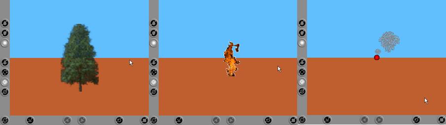
All the elements can be defined using VRML or X3D languaje. The simulator uses a default library with the more common elements needed to repesent the simulation model.
In the next picture, a landscape is shown. This is the initial view of a model, representing the diferent layers that configures the variables. Usually a first layer with the DTM (Digital Terrain Model) is used as a base for all the other layers (vegetation, paths, rivers, etc). Since the model can define different types ofvegetation, different layers representing each one of these layers can be used in the simulation.
|
|
|

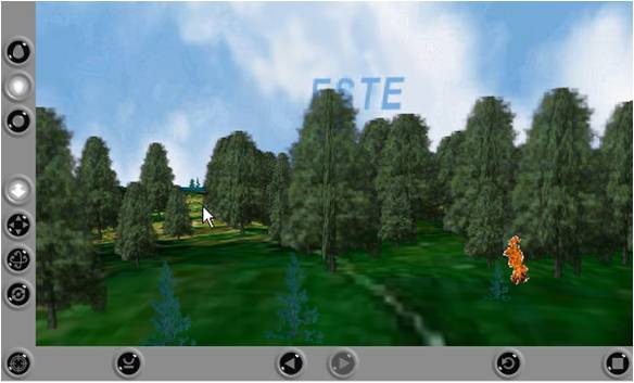
Once the model is configured, the simulation can be executed. A least one point is selected, as the origin of the fire. The simulation engine calculates the fire evolution representing the wildfire as can be viewed in the last picture.

This video shows the execution of a wildfire model.
Once the simulation finish the results can be represented in the virtual reality environment.
The virtual reality model is build using VRML with the Cortona browser embedded in the application.
GISRUK 2006
http://www.nottingham.ac.uk/geography/GISRUK/ 5-7h April 2006, University of Nottingham (UK) |
.jpg) |
GISRUK 2004
http://www.geo.ed.ac.uk/gisruk/gisruk.html 28-30h April 2004, University of East Anglia (Norwich) (UK) |
.jpg) |
Water
Three different researches I conduct regarding water.
Simulation of a river basin
One is related with the flow of the water in a defined environment, representing the river basins and other elements.

Sea level rise
The other research is related with the sea level rise in two different aspects, the representation, and the construction of a model to obtain the new level of the water. In the media section two videos showing the preliminary models are shown.
Black tide
The last research is related with the propagation of a black tide. In the figure is shown a propagation of petroleum over the sea surface using VRML language to represent the model.

Some media
| Here you can see the sea level rise model in the city of New York. The model elevates the water aproximately 100 meters (its not real, here we are testing the web browser infraestructure to represent the simulation model). | |
|
The same model in the city of Barcelona. |
Some publications
If you have a question about the publications please feel free to ask me anything.
ASM 2008
http://iasted.org/conferences/pastinfo-609.html June 23 – 25, 2008 Corfú (Grece) |
|
ASM 2008 Presentation
SDL FORMALIZATION OF A HYDROLOGIC MODEL
Jeaneth López C., Pau Fonseca i Casas, Josep Casanovas
Outline
§ § § § § § Hydrologic Models Simulation Formalisms GIS data Cellular automaton SDL Specification of the model. Discussion
Hydrologic Models
IPCC estimates that there are four places in the earth with high risk to reduce the availability of hydrologic resources and present abrupt climate changes. Spain (south of Europe), California (EEUU), South Africa, North east of
Greenhouse effects
Hydrologic resource
Rise Sea level Natural disastres
•Cyclones •Droughts •Floods •Frost •Etc…
Human Migration
Rise Temperature
Water Availability
Increase of population Precipi tation Contami nation Waste water
Human Consume Agricul ture
Available Water
Industry Ecosystems
Hydro. model – Sim. Formalisms – GIS Data – Cel. Automaton - SDL
Hydrologic Models
Watershed modeling, or hydrologic model (rainfall-runoff modeling) began in the 1950s and 1960s with the evolution of the digital computer. The Stanford Watershed Model (SWM) was one of the first watershed hydrologic model. (Crawford and Linsey 1966). LSSMs (Large-scale Spatial Models)(Watson et al., 1999) DHSVM (Distributed Hydrology-Soil-Vegetation Model) (Wigmosta 1997, 2002) LSHWM (Large-Scale Hybrid Watershed Modeling)(Aral and Gunduz, 2003), MHM (Macroscale Hydrological Model using Variable Infiltration Capacity VIC 3-layer)(Srinivasan2003) The VIC-3L model, is based on a 3-layer Soil Vegetation Atmosphere Transfer scheme to model different surface conditions. L-THIA (Long Term Hydrologic Impacts Assessment) (Lim et al., 2006) Hydrological model SHALL3 (Zimmermann, 2002) (Haan et al.,1982, Singh, 1988, Singh and Frevert, 2006)
Hydro. model – Sim. Formalisms – GIS Data – Cel. Automaton - SDL
Hydrologic Models
The SWAT (Soil and Water Assessment Tool) was developed by modifying the models specified below. All of this models use the SCS Curve Number Method, an empirical formula for predicting runoff from daily rainfall.
GLEAMS
pesticide compone nt daily rainfall hydrology component Crop Growth compone nt
QUAL2 E
Instream kinetics
Example SWAT adaptations
ESWAT SWATG SWIM
SWRRB
(multiple subbasins, subbasins, other other
CREAMS
SWRRB (multiple
SWAT
routing structur e
components)
EPIC
ROTO
Schematic of SWAT developmental history, including selected SWAT
1970s
Hydro. model – Sim. Formalisms – GIS Data – Cel. Automaton - SDL
Nowada ys
Simulation Formalisms
§ Petri Nets
§ Introduced by Carl Adam Petri (1960). Also known as a Place/Transition
§ DEVS (Discreet Event System Specification)
§ In the 70s Bernard Zeigler proposed a mathematical formalism.
§ SDL (Specification and Description Language)
§ The semantics of SDL was defined formally in 1988.
Hydro. model – Sim. Formalisms – GIS Data – Cel. Automaton - SDL
Petri Nets
RdP=(P,T,A,W,M0)
P = Finiteset of nodes Places T = Finiteset of nodes Transitions A C(PxT) and T. (TxP): subset of cartesianproduct between nodes P
W = a {1,2,3,..}: weigh of arcs M0 = Pi {1,2,3,..} node Pi: number ok tokens initials in each place
Hydro. model – Sim. Formalisms – GIS Data – Cel. Automaton - SDL
DEVS Formalism
M=<X, S, Y, δint, δext, λ, ta> where: X: set of input values. S: set of states values. Y: set of output values. δint: internal transition function.
δint :S
S
δext: external transition function. δext Q x X S , on
Q={(s,e)|sS, 0≤e≤ta(s)} set of states. e elapsed time from the last transition.
λ : output function: λ : S Y ta : time advance function.
ta: S
R+0∞
DEVS Processor example
M=<X, S, Y, δint, δext, λ, ta> on: X={job1, job2, .., jobn} S={job1, job2,.., jobn}U[Ø]xR+0∞ Y={y(job1), y(job2),.. Y(jobn)} δint(job,σ)=(Ø, ∞) δext(job,σ,e,x)= if job= Ø (x,tp,(x)) else (job, σ-e) λ(job, σ)=y(job) Ta(job, σ)= σ
SDL formalism
Object-oriented, formal language defined by The International Telecommunications Union as recommendation Z.100. Intended for the specification of complex, event-driven, real-time, and interactive applications involving many concurrent activities that communicate using discrete signals.
Hydro. model – Sim. Formalisms – GIS Data – Cel. Automaton - SDL
SDL Formalism
The semantics of SDL was defined formally in 1988.
Standard Formal Graphical
and symbol-based Object-oriented (OO)
Hydro. model – Sim. Formalisms – GIS Data – Cel. Automaton - SDL
GIS Data
Hydro. model – Sim. Formalisms – GIS Data – Cel. Automaton - SDL
Celular automaton
Each cell xi(t) represent a state of the cell i in the instant t. k = {Empty, Static and Dynamic}
xi
Hydro. model – Sim. Formalisms – GIS Data – Cel. Automaton - SDL
Game of life
The Game of Life is a cellular automaton devised by the British mathematician John Horton Conway in 1970. It is the best-known example of a cellular
Hydro. model – Sim. Formalisms – GIS Data – Cel. Automaton - SDL
Method
§ Cellular Automaton Structure
§ Evolution Rules
§ Precipitation phase § Settlement phase
• Data layers
Hydro. model – Sim. Formalisms – GIS Data – Cel. Automaton - SDL
Model
Soil (Ground)
•Return Flow •Kind of soil •Saturate •Kind of soil use •Non-Saturate •Percolation
•Runoff •Humidity •Evapo-trans piration •Temperature •Rainfall •Precipitation
Hydrologic resource
Meteorology
Factors/variables which affects hydrologic resource
Hydro. model – Sim. Formalisms – GIS Data – Cel. Automaton - SDL
Model
Where:
SWt is the total quantity of water in the soil (basin) (mm), SWi is the initial quantity of water in the soil (mm) Ri (rainfall) is the quantity of rain in the period of analysis(mm) Qi is the quantity of runoff (mm) ETi is the evapotranspiration (mm) Pi is the percolation (mm) QRi return flow(mm) t is the time expressed in days i is the index of cell
Hydro. model – Sim. Formalisms – GIS Data – Cel. Automaton - SDL
Model
This expression gives us the water volume existing in each cell of our cellular automaton in a specific time t. In the expression, one position of the cellular automaton matrix [xi,xj] is represented by the cell xi.
Hydro. model – Sim. Formalisms – GIS Data – Cel. Automaton - SDL
System diagram
Hydro. model – Sim. Formalisms – GIS Data – Cel. Automaton - SDL
States diagram
Update Receive
Send
Dynamic
Receiv e
Static
d en S te/ ei ec R ve
Update Receive
Receive
Send
Up
da
Send Update
Empty
Hydro. model – Sim. Formalisms – GIS Data – Cel. Automaton - SDL
Process diagram: Static state
Hydro. model – Sim. Formalisms – GIS Data – Cel. Automaton - SDL
Process diagram: Empty state
Hydro. model – Sim. Formalisms – GIS Data – Cel. Automaton - SDL
Process diagram: Dynamic state
Hydro. model – Sim. Formalisms – GIS Data – Cel. Automaton - SDL
Discussion and future work
This slides depicts the first and more important step to construct a discrete hydrologic simulator based in a cellular automaton. It shows the specification of hydrologic model with the aim of simulate the behaviour of water in a river basin. The use of the cellular simplifies the mathematical expressions and helps us to maintain a structured view of the geographical data needed to represent the model. The use of SDL formalism simplifies the understanding of the behaviour of model thanks its graphical structure. The model is based in the hydrologic balance equation which permits calculate the quantity exist in each cell of the cellular automaton
Hydro. model – Sim. Formalisms – GIS Data – Cel. Automaton - SDL
References
[1] L. Ma, L.R. Ahuja, and R.W. Malone. Systems Modeling for Soil and Water Research and Management: Current Status and Needs for the 21st Century. ASABE, 1907-2007. [2] IPCC Intergovernamental Panel on Climate Change. Report IPCC. 2007. [3] J. Samper, M.A. Garcia, B. Pisani, D. Alvares, A. Varela, and J.A. Losada. Modelos Hidrologicos y Sistemas de Informacion Geografica para la Estimacion de Recursos Hidricos:. Confederacin Hidrologica del Ebro, VII, 2005. [4] E. Guzman, J. Bonini, and D. Matamoros. Modelo Hidrologico SWAT (Soil Water Assessment Tool) Prediccin de Caudales y Sedimentos en una Cuenca. Revista Tecnologica, 17:152–161, 2004. [5] Erik D. Zimmermann. Modelo Hidrologico Superficial y Subterraneo. Centro Universitario rosario de Investigaciones Hidroambientales. [6] A. López, D. Sauri, and Jose M. Galán. Urban Water
References
[8] P. Pea and J. Alirio. Sobre las redes de petri r-difusas. Divulgaciones Matemticas, 7:87–99, 1999. [9] Gabriel Wainer. Applying cell-devs methodology for modeling the environment. SIMULATION, 82:635, 2006. [10] Liu Qi and Gabriel Wainer. Parallel environment for devs and cell-devs models. SIMULATION, 83:449, 2007. [11] Fonseca P. and Casanovas J. 2005. ESS205, Simplifying GIS data use inside discrete event simulation model through m_n-AC cellular automaton; Proceedings ESS 2005. [12] ITU-T Telecommunication Standardization Sector of ITU. Languages and general software aspects for telecommunication systems. TELECOMMUNICATION STANDARDIZATION SECTOR OF ITU, 2007. [13] Zeigler, B. P.; H. Praehofer; D. Kim. 2000. Theory of Modeling and Simulation. Academic Press. [14] Petri, Carl A. 1962. "Kommunikation mit Automaten". Ph. D. Thesis. University of Bonn. [15] Recalde, L.; Teruel, E.; Silva, M. 1999. Autonomous
Thanks!
Pau Fonseca i Casas pau@fib.upc.edu
Technical University of Catalonia Barcelona School of Informatics Computing laboratory Barcelona Jordi Girona 1-3 (+34)93401773
The financial market experiment
We present an experiment that aims to simulate the figure of the broker, from the point of view of human behavior adding hunches and expectations too its decisions. As a starting point we use the paper of Veiga and Vorsatz, "Price manipulation in an experimental asset market”, a study that analyzes the influence on the behavior the other brokers due to an agent handle and a trading robot that performs with the intention of distort the market and thus, try to profit from their operations. In this research conducted by Veiga and Vorsatz, it is required the participation of real people whit the aim of analyze the behavior of the process of buying and selling a value in two separate rooms, one with the influence of manipulative agent and another without it. This article reproduces this experiment but using virtual brokers that belongs to a multi-agent simulation model. The main objective is to reproduce the experiment represented in the Veiga and Vorsatz paper using intelligent agents detailing the description of the psychological behavior of the brokers.
To execute the models you must download the zip files, extract it on a folder and execute the SDLPS engine. The file that rules the behavior of the model is SimBroker.sdlps. This file contains all the details of both models.
Remember that SDLPS can only be used to execute the models or for academic purposes. (POSAR LA LLICÈNCIA FORMAT UPC).
| Attachment | Size |
|---|---|
| Low hunches model | 26.62 MB |
| SDLPS simulator | 31.04 MB |